NeRF: A Volume Rendering Perspective

Overview

NeRF implicitly represents a 3D scene with a multi-layer perceptron (MLP) $F: (\boldsymbol{x}, \boldsymbol{d}) \rightarrow (\boldsymbol{c}, \sigma)$ for some position $\boldsymbol{x} \in \mathbb{R}^3$, view direction $\boldsymbol{d} \in [0, \pi) \times [0, 2\pi)$, color $\boldsymbol{c}$, and "opacity" $\sigma$. Rendered results are spectacular.

There have been a number of articles introducing NeRF since its publication in 2020. While most posts mention general methods, few of them elaborate on why the volume rendering procedure

$$\mathbf{C}(\boldsymbol{r}) = \gray{\mathbf{C}(z; \boldsymbol{o}, \boldsymbol{d}) =} \int_{z_n}^{z_f} T\gray{(z)} \sigma \left( \boldsymbol{r}\gray{(z)} \right) \boldsymbol{c} \left(\boldsymbol{r}\gray{(z)}, \boldsymbol{d} \right) \ dz, \ T(z) = \exp \left(-\int_{z_n}^z \sigma \left(\boldsymbol{r} \gray{(s)} \right) \ ds \right)$$

for a ray $\boldsymbol{r} = \boldsymbol{o} + z\boldsymbol{d}$ works and how the equation is reduced to

$$\hat{\mathbf{C}}(\boldsymbol{r}) = \gray{\hat{\mathbf{C}}(z_1, z_2, \ldots, z_N; \boldsymbol{o}, \boldsymbol{d}) =} \sum_{i=1}^{N} T_i \left(1 - e^{-\sigma_i \delta_i} \right) \boldsymbol{c}_i, \ T_i = \exp \left(-\sum_{j=1}^{i-1} \sigma_j \delta_j \right)$$

via numerical quadrature, let alone exploring its implementation via Monte Carlo method.

This post delves into the volume rendering aspect of NeRF. The equations will be derived; its implementation will be analyzed.

Prerequisites

• Having read the NeRF paper
• Ability to solve ordinary differential equations (ODEs)
• Introductory probability theory
• Familiarity with PyTorch and NumPy

Background

The rendering formula

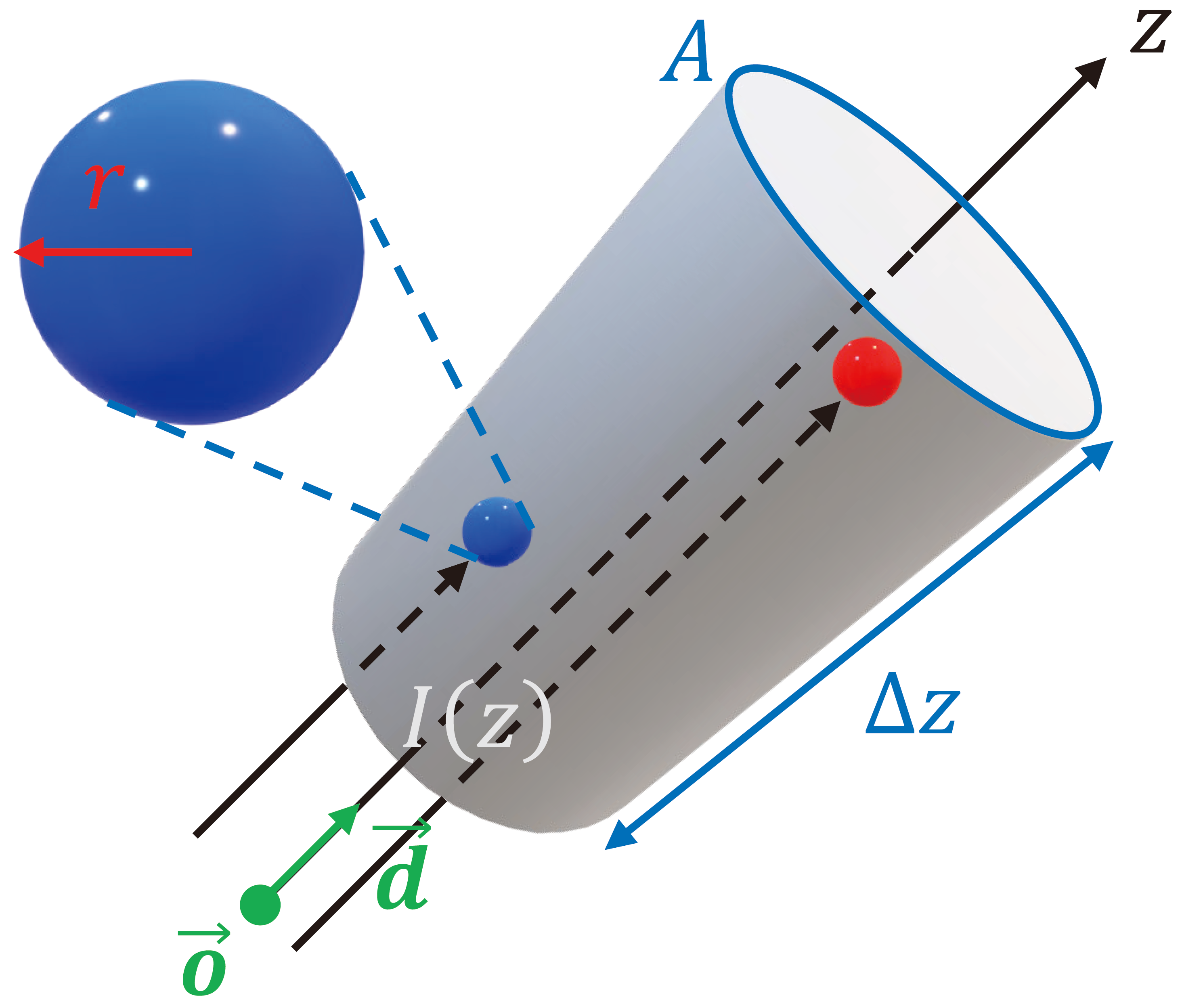
A ray with origin $\boldsymbol{o}$ and direction $\boldsymbol{d}$ casts to an arbitrary region of bounded space. Assume, for simplicity, that the cross section area $A$ is uniform along the ray. Let's focus on a slice of the region with thickness $\Delta z$.

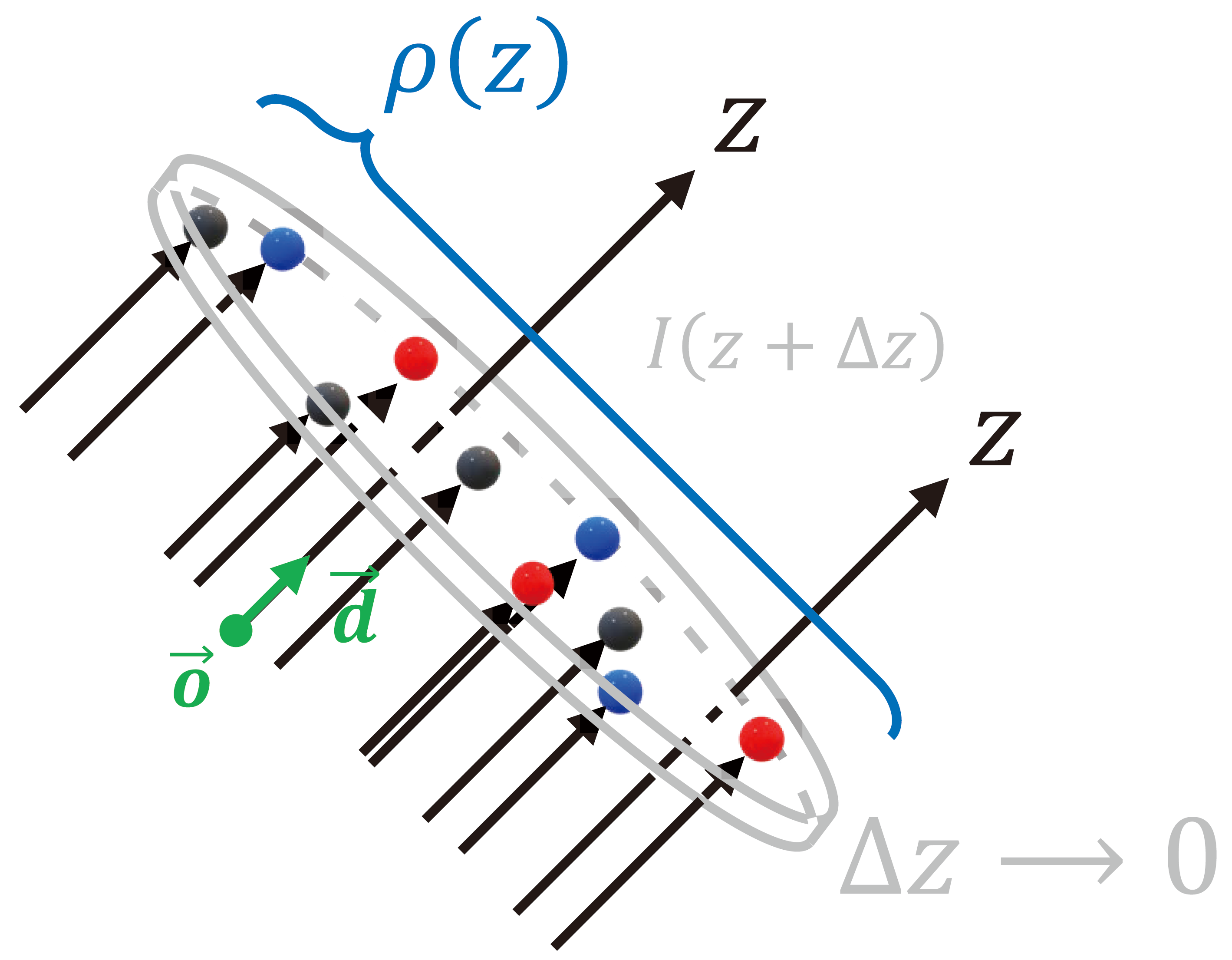
Occluding objects are modeled as spherical particles with radius $r$. Let $\rho(z\gray{; \boldsymbol{o}, \boldsymbol{d}})$ denote the particle density — number of particles per unit volume — in that orientation. If $\Delta z$ is small enough such that $\rho(z)$ is consistent on the slice, then there are

$$\underbrace{A \cdot \Delta z}_\text{slice volume} \cdot \rho(z)$$

particles contained in the slice. When $\Delta z \rightarrow 0$, solid particles do not overlap, then a total of

$$\underbrace{A \cdot \Delta z}_\text{slice volume} \cdot \rho(z) \cdot \underbrace{\pi r^2}_\text{particle area}$$

area is occluded, which amounts to a portion of $\frac{A \Delta z \cdot \rho(z) \cdot \pi r^2}{A} = \pi r^2 \rho(z) \Delta z$ of the cross section. Let $I(z\gray{; \boldsymbol{o}, \boldsymbol{d}})$ denote the light intensity at depth $z$ from origin $\boldsymbol{o}$ along direction $\boldsymbol{d}$. If a portion of $\pi r^2 \rho(z) \Delta z$ of all rays are occluded, then the intensity at depth $z + \Delta z$ decreases to

$$I(z + \Delta z) = (1 - \underbrace{\pi r^2 \rho(z) \Delta z}_\text{occluded portion})I(z)$$

The difference in intensity is

$$\begin{align*} \Delta I &= I(z + \Delta z) - I(z) \\ &= -\pi r^2 \rho(z) \Delta z \ I(z) \end{align*}$$

Take a step from discrete to continuous, we have

$$dI(z) = - \underbrace{\pi r^2 \rho(z)}_{\sigma(z)} I(z) \ dz$$

Define volume density (or voxel "opacity") $\sigma(z\gray{; \boldsymbol{o}, \boldsymbol{d}}) := \pi r^2 \rho(z\gray{; \boldsymbol{o}, \boldsymbol{d}})$. This makes sense because the amount of ray reduction depends on both the number of occluding particles and the size of them, then the solution to the ODE

$$dI(z) = -\sigma(z) I(z) \ dz$$

is

$$I(z) = I(z_0) \ \underbrace{e^{\int_{z_0}^{z} -\sigma(s) \ ds}}_{T(z)}$$

Step-by-step solution

Exchange the terms at both sides of the ODE:

$$\frac{1}{I(z)} \ dI(z) = -\sigma(z) \ dz$$

which is a separable DE. Integrate both sides

$$\begin{align*} \int \frac{1}{I(z)} \ dI(z) &= \int -\sigma(z) \ dz \\ \ln I(z) &= \int -\sigma(z) \ dz + C \\ I(z) &= C e^{\int -\sigma(z) \ dz} \end{align*}$$

Suppose $I$ takes $I(z_0)$ at depth $z_0$, then

$$I(z) = I(z_0) \ e^{\int_{z_0}^{z} -\sigma(s) \ ds}$$

Define accumulated transmittance $T(z) := e^{\int_{z_0}^{z} -\sigma(s) \ ds}$, then $I(z) = I(z_0)T(z)$ means the remainning intensity after the rays travels from $z_0$ to $z$. $T(z)$ can also be viewed as the cumulative density function (CDF) that a ray does not hit any particles from $z_0$ to $z$. But no color will be observed if a ray passes empty space; radiance is "emitted" only when there is contact between rays and particles. Define

$$H(z) := 1 - T(z)$$

as the CDF that a ray hits particles from $z_0$ to $z$, then its probability density function (PDF) is

$$p_\text{hit}(z) = -\underbrace{e^{\int_{z_0}^{z} -\sigma(s) \ ds}}_{T(z)} \ \sigma(z)$$

CDF to PDF

Differentiate CDF $H(z)$ (w.r.t. $z$) to get $p_\text{hit}(z)$

$$\begin{align*} p_\text{hit}(z) &= \frac{dH}{dz} \\ &= -\frac{dT}{dz} \\ &= -\frac{d}{dz} e^{\int_{z_0}^{z} -\sigma(s) \ ds} \\ &= -e^{\int_{z_0}^{z} -\sigma(s) \ ds} \ \frac{d}{dz} \int_{z_0}^{z} -\sigma(s) \ ds \\ &= -e^{\int_{z_0}^{z} -\sigma(s) \ ds} \ \sigma(z) \end{align*}$$

Let a random variable a random variable $\mathbf{R}$ denote the emitted radiance, then

$$\begin{align*} p_{\mathbf{R}}\gray{(\boldsymbol{r})} =& \ p_{\mathbf{R}}\gray{(z; \boldsymbol{o}, \boldsymbol{d})} \\ :=& \ P[\mathbf{R} = \boldsymbol{c}\gray{(z)}] \\ =& \ p_\text{hit}\gray{(z)} \end{align*}$$

Hence, the color of a pixel is the expectation of emitted radiance:

$$\begin{align*} \mathbf{C}(\boldsymbol{r}) \gray{= \mathbf{C}(z; \boldsymbol{o}, \boldsymbol{d})} &= \mathbb{E} (\mathbf{R}) \\ &= \int_0^\infty \mathbf{R} \ p_{\mathbf{R}} \ dz \\ &= \int_0^\infty \boldsymbol{c} \ p_\text{hit} \ dz \\ &= \int_0^\infty T(z) \sigma(z) \boldsymbol{c}(z) \ dz \end{align*}$$

concluding the proof.

Integration bounds

In practice, $\boldsymbol{c}$, obtained from MLP query, is a function of both position $z$ (or coordinate $\boldsymbol{x}$) and view direction $\boldsymbol{d}$. Also different are the integration bounds. A computer does not support an infinite range; the lower and upper bounds of integration are $z_\text{n\gray{ear}} = \verb|near|$ and $z_\text{f\gray{ar}} = \verb|far|$ within the range of floating point representation:

$$\mathbf{C}(\boldsymbol{r}) = \int_\verb|near|^\verb|far| T(z) \sigma(z) \boldsymbol{c}(z) \ dz$$

In NeRF, $\verb|near| =$ 0. and $\verb|far| =$ 1. for scaled bounded scenes and front facing scenes after conversion to normalized device coordinates (NDC).

Numerical quadrature

We took a step from discrete to continuous to derive the rendering integral. Nevertheless, integration on a continuous domain is not supported by computers. An alternative is numerical quadrature. Sample $\verb|near| \lt z_1 \lt z_2 \lt \cdots \lt z_{N} \lt \verb|far|$ along a ray, and define differences between adjacent samples as

$$\delta_i := z_{i+1} - z_i \ \forall i \in \{1,\ldots,N-1\}$$

then the transmittance is approximated by

$$\begin{align*} T_i :=&\ T(z_i) \\ \approx&\ e^{-\sum_{j=1}^{i\blue{-1}} \sigma_j \delta_j} \end{align*}$$

where $T_1 = 1$ and $\sigma_j = \sigma(z_j\gray{; \boldsymbol{o}, \boldsymbol{d}})$. Meanwhile, differentiation in $p_\text{hit}(z)$ is also substituted by discrete difference. That is,

$$\begin{align*} p_i := p_\text{hit}(z_i) &= \left. \frac{dH}{dz} \right|_{z_i} \\ &\approx H(z_{i+1}) - H(z_i) \\ &\gray{= 1- T(z_{i+1}) - \left(1- T(z_i)\right)} \\ &= T(z_i) - T(z_{i+1}) \\ &= T_i \left(1 - e^{-\sigma_i \delta_i}\right) \end{align*}$$

Step-by-step solution

$$\begin{align*} T(z_i) - T(z_{i+1}) &= T(z_i) \left(1 - \frac{T(z_{i+1})}{T(z_i)}\right) \\ &= T(z_i) \left( 1 - \frac{e^{-\sum_{j=1}^{\green{i}} \sigma_j \delta_j}}{e^{-\sum_{j=1}^{\blue{i-1}} \sigma_j \delta_j}} \right) \\ &= T(z_i) \left(1 - e^{-\sum_{j=1}^{\green{i}} \sigma_j \delta_j + \sum_{j=1}^{\blue{i-1}} \sigma_j \delta_j}\right) \\ &= T_i \left(1 - e^{-\sigma_{\green{i}} \delta_{\green{i}}}\right) \end{align*}$$

Hence, the discretized emmitted radiance is

$$\begin{align*} \hat{\mathbf{C}}(\boldsymbol{r}) \gray{= \hat{\mathbf{C}}(z; \boldsymbol{o}, \boldsymbol{d})} &= \mathbb{E} (\mathbf{R}) \\ &= \int_\verb|near|^\verb|far| \mathbf{R} \ p_{\mathbf{R}} \ dz \\ &\approx \sum_{i=1}^N \boldsymbol{c}_i T_i \left(1 - e^{-\sigma_i \delta_i}\right) \end{align*}$$

where $\boldsymbol{c}_i := \boldsymbol{c}(z_i\gray{; \boldsymbol{o}, \boldsymbol{d}})$ is the output RGB upon MLP query at $\{z_i \ | \ \boldsymbol{o}, \boldsymbol{d}\}$.

Note that if we denote $\alpha_i := 1 - e^{-\sigma_i \delta_i}$, then $\hat{\mathbf{C}}(\boldsymbol{r}) = \sum_{i=1}^N \alpha_i T_i \boldsymbol{c}_i$ resembles classical alpha compositing.

Alpha compositing

Consider the case where a foreground object is inserted ahead of the background. Now that a pixel displays a single color, we have to blend the colors of the two. Compositing is applied when there are partially transparent regions within the foreground object, or the foreground object partially covers the background.

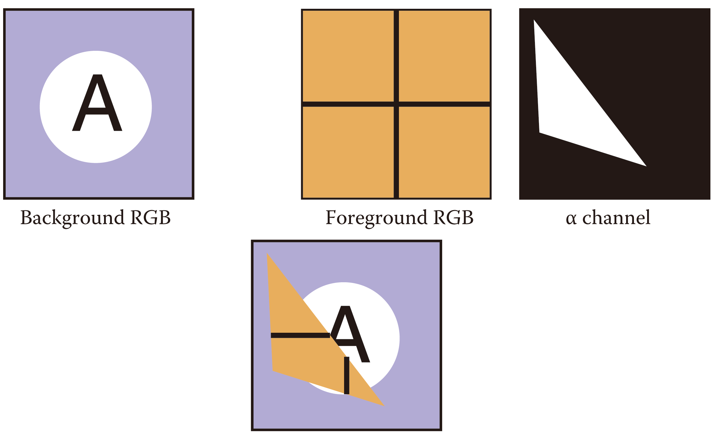
In alpha compositing, a parameter $\alpha$ determines the extent to which each object contributes to what is displayed in a pixel. Let $\alpha$ denote the opacity (or pixel coverage) of the foreground object, then a pixel showing foreground color $\boldsymbol{c}_f$ over background color $\boldsymbol{c}_b$ is composited as

$$\boldsymbol{c} = \alpha \boldsymbol{c}_f + (1 - \alpha) \boldsymbol{c}_b$$

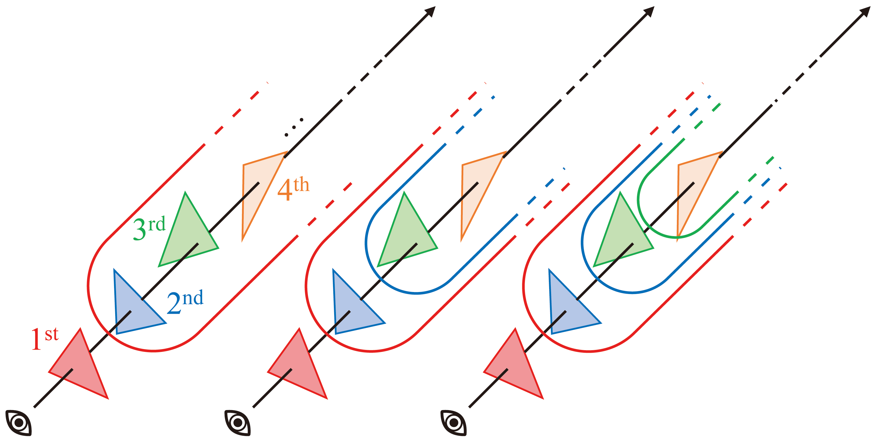
When blending colors of multiple objects, one can adopt a divide-and-conquer approach. Each time, cope with the unregistered object closest to the eye and treat the remaining objects as a single entity. Such a strategy is formulated by

$$\begin{align*} \boldsymbol{c} &= \red{\alpha_1 \boldsymbol{c}_1} + (1 - \red{\alpha_1})\biggl( \blue{\alpha_2 \boldsymbol{c}_2} + \left( 1 - \blue{\alpha_2} \right)\Bigl( \green{\alpha_3 \boldsymbol{c}_3} + \left( 1 - \green{\alpha_3} \right)\bigl( \orange{\alpha_4 \boldsymbol{c}_4} + (1 - \orange{\alpha_4})\left( \cdots \right) \bigr) \Bigr) \biggr) \\ &= \red{\alpha_1 \boldsymbol{c}_1} + (1 - \red{\alpha_1})\blue{\alpha_2 \boldsymbol{c}_2} \\ & \ \ \ \ \ \ \ \ \ \ \ \ \ + (1 - \red{\alpha_1})( 1 - \blue{\alpha_2})\Bigl( \green{\alpha_3 \boldsymbol{c}_3} + \left( 1 - \green{\alpha_3} \right)\bigl( \orange{\alpha_4 \boldsymbol{c}_4} + (1 - \orange{\alpha_4})\left( \cdots \right) \bigr) \Bigr) \\ &= \red{\alpha_1 \boldsymbol{c}_1} + (1 - \red{\alpha_1})\blue{\alpha_2 \boldsymbol{c}_2} \\ & \ \ \ \ \ \ \ \ \ \ \ \ \ + (1 - \red{\alpha_1})(1 - \blue{\alpha_2})\green{\alpha_3 \boldsymbol{c}_3} \\ & \ \ \ \ \ \ \ \ \ \ \ \ \ + (1 - \red{\alpha_1})(1 - \blue{\alpha_2})(1 - \green{\alpha_3})\bigl( \orange{\alpha_4 \boldsymbol{c}_4} + (1 - \orange{\alpha_4})\left( \cdots \right) \bigr) \\ &= \red{\alpha_1 \boldsymbol{c}_1} + (1 - \red{\alpha_1})\blue{\alpha_2 \boldsymbol{c}_2} \\ & \ \ \ \ \ \ \ \ \ \ \ \ \ + (1 - \red{\alpha_1})(1 - \blue{\alpha_2}) \green{\alpha_3 \boldsymbol{c}_3} \\ & \ \ \ \ \ \ \ \ \ \ \ \ \ + (1 - \red{\alpha_1})(1 - \blue{\alpha_2})(1 - \green{\alpha_3})\orange{\alpha_4 \boldsymbol{c}_4} \\ & \ \ \ \ \ \ \ \ \ \ \ \ \ + (1 - \red{\alpha_1})(1 - \blue{\alpha_2})(1 - \green{\alpha_3})(1 - \orange{\alpha_4})\left( \cdots \right) \\ &= \cdots \end{align*}$$

which is essentially a tail recursion.

Alpha compositing in NeRF

There are $N$ samples along each ray in NeRF. Consider the first $N - 1$ samples as occluding foreground objects with opacity $\alpha_i$ and color $\boldsymbol{c}_i$, and the last sample as background, then the blended pixel value is

$$\begin{align*} \tilde{\mathbf{C}} &= \alpha_1 \boldsymbol{c}_1 + (1 - \alpha_1) \alpha_2 \boldsymbol{c}_2 \\ & \ \ \ \ \ \ \ \ \ \ \ \ \ + (1 - \alpha_1)(1 - \alpha_2) \alpha_3 \boldsymbol{c}_3 \\ & \ \ \ \ \ \ \ \ \ \ \ \ \ + (1 - \alpha_1)(1 - \alpha_2)(1 - \alpha_3) \alpha_4 \boldsymbol{c}_4 \\ & \ \ \ \ \ \ \ \ \ \ \ \ \ \cdots \\ & \ \ \ \ \ \ \ \ \ \ \ \ \ + (1 - \alpha_1)(1 - \alpha_2)(1 - \alpha_3) \cdots (1 - \alpha_{N-1}) \boldsymbol{c}_N \\ &= \sum_{i=1}^{N} \left(\alpha_i \boldsymbol{c}_i \prod_{j=1}^{i-1} \left(1 - \alpha_j\right)\right) \end{align*}$$

where $\alpha_0 = 0$. Recall $\hat{\mathbf{C}} = \sum_{i=1}^N \alpha_i T_i \boldsymbol{c}_i$, then it remains to show that $\prod_{j=1}^{i-1} \left(1 - \alpha_j\right) = T_i$:

$$\begin{align*} \prod_{j=1}^{i-1} \left(1 - \alpha_j\right) &= \prod_{j=1}^{i-1} e^{-\sigma_j \delta_j} \\ &= \exp \left( \sum_{j=1}^{i-1} -\sigma_j \delta_j \right) \\ &= T_i \end{align*}$$

concluding the proof. This manifests the elegancy of differentiable volume rendering.

Rewrite $w_i := \alpha_i T_i$, then the expectation of emmitted radiance $\mathbf{C}(\boldsymbol{r}) = \sum_{i=1}^N w_i \boldsymbol{c}_i$ is weighted sum of colors.

Why (trivially) differentiable?

Given the above renderer, a coarse training pipeline is

$$\left. \begin{array}{r} \text{ground truth} \ \mathbf{C} \\ (\boldsymbol{x}, \boldsymbol{d}) \xrightarrow{\text{MLP}} (\boldsymbol{c}, \sigma) \xrightarrow{\text{discrete rendering}} \text {prediction} \ \hat{\mathbf{C}} \end{array} \right\} \xrightarrow{\text{MSE}} \mathcal L = \| \hat{\mathbf{C}} - \mathbf{C} \|_{\gray{2}}^2$$

If the discrete renderer is differentiable, then we can train the end-to-end model through gradient descent. No suprise, given a (sorted) sequence of random samples $\boldsymbol{t} = \{t_1, t_2, \ldots, t_N\}$, the derivatives are

$$\begin{align*} \left. \frac{d \hat{\mathbf{C}}}{d \boldsymbol{c}_i} \right|_{\boldsymbol{t}} &= T_i \left(1 - e^{-\sigma_i \delta_i} \right) \\ \left. \frac{d \hat{\mathbf{C}}}{d \sigma_i} \right|_{\boldsymbol{t}} &= \boldsymbol{c}_i \left( \green{\frac{d T_i}{d \sigma_i}} \blue{\left( 1 - e^{-\sigma_i \delta_i} \right)} + \green{T_i} \blue{\frac{d}{d \sigma_i} \left( 1 - e^{-\sigma_i \delta_i} \right)} \right) \\ &= \mathbf{c}_i \left( \blue{\left( 1 - e^{-\sigma_i \delta_i} \right)} \green{\exp \left(-\sum_{j=1}^{i-1} \sigma_j \delta_j \right)} \underbrace{\green{\frac{d}{d \sigma_i} \left( -\sum_{j=1}^{i-1} \sigma_j \delta_j \right)}}_{0} + \green{T_i} \blue{\left( -e^{-\sigma_i \delta_i} \right) \frac{d(-\sigma_i \delta_i)}{d \sigma_i}} \right) \\ &= \delta_i T_i \boldsymbol{c}_i e^{-\sigma_i \delta_i} \end{align*}$$

Once the renderer is differentiable, weights and biases in an MLP can be updated via the chain rule.

Coarse-to-fine approach

NeRF jointly optimizes coarse and fine network.

Analysis

Whereas NeRF is originally implemented in Tensrorflow, code analysis is based on a faithful reproduction in PyTorch. The repository is organized as

Let's experiment with the LLFF dataset, which is comprised of front-facing scenes with camera poses. Pertinent directories and files are

Item	Type	Description
configs	directory	contains per scene configuration (.txt) for the LLFF dataset
download_example_data.sh	shell script	to download datasets
load_llff.py	Python script	data loader of the LLFF dataset
run_nerf.py	Prthon script	main procedures
run_nerf_helpers.py	Python script	utility functions

Modified identation and comments

Codes in this post deviate slightly from the authentic version. Dataflow and function calls remain intact whereas indentation and comments are modified for the sake of readibility.

The big picture

if __name__ == '__main__':
    torch.set_default_tensor_type('torch.cuda.FloatTensor')
    train()

As shown, train(…) in run_nerf.py is the execution entry to the project. The entire training process is

def train():

    parser = config_parser()
    args = parser.parse_args()

    # load data
    K = None
    if args.dataset_type == 'llff':
        images, poses, bds, render_poses, i_test = load_llff_data(args.datadir, args.factor,
                                                                  recenter=True, bd_factor=.75,
                                                                  spherify=args.spherify)
        hwf = poses[0,:3,-1]
        poses = poses[:,:3,:4]
        print('Loaded llff', images.shape, render_poses.shape, hwf, args.datadir)
        if not isinstance(i_test, list):
            i_test = [i_test]

        if args.llffhold > 0:
            print('Auto LLFF holdout,', args.llffhold)
            i_test = np.arange(images.shape[0])[ : :args.llffhold]

        i_val = i_test
        i_train = np.array([i for i in np.arange(int(images.shape[0]))
                                  if (i not in i_test and i not in i_val)])

        print('DEFINING BOUNDS')
        if args.no_ndc:
            near = np.ndarray.min(bds) * .9
            far = np.ndarray.max(bds) * 1.
            
        else:
            near = 0.
            far = 1.
        print('NEAR FAR', near, far)

    elif args.dataset_type == 'blender':
        images, poses, render_poses, hwf, i_split = load_blender_data(args.datadir, args.half_res, args.testskip)
        print('Loaded blender', images.shape, render_poses.shape, hwf, args.datadir)
        i_train, i_val, i_test = i_split

        near = 2.
        far = 6.

        if args.white_bkgd:
            images = images[...,:3]*images[...,-1:] + (1.-images[...,-1:])
        else:
            images = images[...,:3]

    elif args.dataset_type == 'LINEMOD':
        images, poses, render_poses, hwf, K, i_split, near, far = load_LINEMOD_data(args.datadir, args.half_res, args.testskip)
        print(f'Loaded LINEMOD, images shape: {images.shape}, hwf: {hwf}, K: {K}')
        print(f'[CHECK HERE] near: {near}, far: {far}.')
        i_train, i_val, i_test = i_split

        if args.white_bkgd:
            images = images[...,:3]*images[...,-1:] + (1.-images[...,-1:])
        else:
            images = images[...,:3]

    elif args.dataset_type == 'deepvoxels':

        images, poses, render_poses, hwf, i_split = load_dv_data(scene=args.shape,
                                                                 basedir=args.datadir,
                                                                 testskip=args.testskip)

        print('Loaded deepvoxels', images.shape, render_poses.shape, hwf, args.datadir)
        i_train, i_val, i_test = i_split

        hemi_R = np.mean(np.linalg.norm(poses[:,:3,-1], axis=-1))
        near = hemi_R-1.
        far = hemi_R+1.

    else:
        print('Unknown dataset type', args.dataset_type, 'exiting')
        return

    # cast intrinsics to right types
    H, W, focal = hwf
    H, W = int(H), int(W)
    hwf = [H, W, focal]

    if K is None:
        K = np.array([
            [focal, 0    , 0.5*W],
            [0    , focal, 0.5*H],
            [0    , 0    , 1    ]
        ])

    if args.render_test:
        render_poses = np.array(poses[i_test])

    # create log dir and copy the config file
    basedir = args.basedir
    expname = args.expname
    os.makedirs(os.path.join(basedir, expname), exist_ok=True)
    f = os.path.join(basedir, expname, 'args.txt')
    with open(f, 'w') as file:
        for arg in sorted(vars(args)):
            attr = getattr(args, arg)
            file.write('{} = {}\n'.format(arg, attr))
    if args.config is not None:
        f = os.path.join(basedir, expname, 'config.txt')
        with open(f, 'w') as file:
            file.write(open(args.config, 'r').read())

    # create nerf model
    render_kwargs_train, render_kwargs_test, start, grad_vars, optimizer = create_nerf(args)
    global_step = start

    bds_dict = {'near': near,
                'far' : far}
    render_kwargs_train.update(bds_dict)
    render_kwargs_test.update(bds_dict)

    # move test data to GPU
    render_poses = torch.Tensor(render_poses).to(device)

    # short circuit if rendering from trained model
    if args.render_only:
        print('RENDER ONLY')
        with torch.no_grad():
            if args.render_test:
                images = images[i_test] # switch to test poses
            else:
                # default is smoother render_poses path
                images = None

            testsavedir = os.path.join(basedir, expname, 'renderonly_{}_{:06d}'.format('test' if args.render_test else 'path', start))
            os.makedirs(testsavedir, exist_ok=True)
            print('test poses shape', render_poses.shape)

            rgbs, _ = render_path(render_poses, hwf, K, args.chunk, render_kwargs_test, gt_imgs=images, savedir=testsavedir, render_factor=args.render_factor)
            print('Done rendering', testsavedir)
            imageio.mimwrite(os.path.join(testsavedir, 'video.mp4'), to8b(rgbs), fps=30, quality=8)

            return

    # prepare raybatch tensor if batching random rays
    N_rand = args.N_rand
    use_batching = not args.no_batching
    if use_batching:
        # random ray batching
        print('get rays')
        rays = np.stack([get_rays_np(H, W, K, p) for p in poses[:,:3,:4]], 0) # (num_img, ro+rd, H, W, 3)
        print('done, concats')
        rays_rgb = np.concatenate([rays, images[:,None]], 1) # (num_img, ro+rd+rgb, H, W, 3)
        rays_rgb = np.transpose(rays_rgb, [0,2,3,1,4]) # (num_img, H, W, ro+rd+rgb, 3)
        rays_rgb = np.stack([rays_rgb[i] for i in i_train], 0) # training set only
        rays_rgb = np.reshape(rays_rgb, [-1,3,3]) # ((num_img-1)*H*W, ro+rd+rgb, 3)
        rays_rgb = rays_rgb.astype(np.float32)
        print('shuffle rays')
        np.random.shuffle(rays_rgb)

        print('done')
        i_batch = 0

    # move training data to GPU
    if use_batching:
        images = torch.Tensor(images).to(device)
    poses = torch.Tensor(poses).to(device)
    if use_batching:
        rays_rgb = torch.Tensor(rays_rgb).to(device)


    N_iters = 200000 + 1
    print('Begin')
    print('TRAIN views are', i_train)
    print('TEST views are', i_test)
    print('VAL views are', i_val)

    # summary writers
    #writer = SummaryWriter(os.path.join(basedir, 'summaries', expname))
    
    start = start + 1
    for i in trange(start, N_iters):
        time0 = time.time()

        # sample random ray batch
        if use_batching:
            # random over all images
            batch = rays_rgb[i_batch:i_batch+N_rand] # (B, 2+1, 3*?)
            batch = torch.transpose(batch, 0, 1)
            batch_rays, target_s = batch[:2], batch[2]

            i_batch += N_rand
            if i_batch >= rays_rgb.shape[0]:
                print("Shuffle data after an epoch!")
                rand_idx = torch.randperm(rays_rgb.shape[0])
                rays_rgb = rays_rgb[rand_idx]
                i_batch = 0
        else:
            # random from one image
            img_i = np.random.choice(i_train)
            target = images[img_i]
            target = torch.Tensor(target).to(device)
            pose = poses[img_i, :3,:4]

            if N_rand is not None:
                rays_o, rays_d = get_rays(H, W, K, torch.Tensor(pose))  # (H, W, 3), (H, W, 3)

                if i < args.precrop_iters:
                    dH = int(H//2 * args.precrop_frac)
                    dW = int(W//2 * args.precrop_frac)
                    coords = torch.stack(
                        torch.meshgrid(
                            torch.linspace(H//2 - dH, H//2 + dH - 1, 2*dH), 
                            torch.linspace(W//2 - dW, W//2 + dW - 1, 2*dW)
                        ), -1)
                    if i == start:
                        print(f"[Config] Center cropping of size {2*dH} x {2*dW} is enabled until iter {args.precrop_iters}")                
                else:
                    coords = torch.stack(torch.meshgrid(torch.linspace(0, H-1, H), torch.linspace(0, W-1, W)), -1)  # (H, W, 2)

                coords = torch.reshape(coords, [-1,2])  # (H * W, 2)
                select_inds = np.random.choice(coords.shape[0], size=[N_rand], replace=False)  # (N_rand,)
                select_coords = coords[select_inds].long()  # (N_rand, 2)
                rays_o = rays_o[select_coords[:, 0], select_coords[:, 1]]  # (N_rand, 3)
                rays_d = rays_d[select_coords[:, 0], select_coords[:, 1]]  # (N_rand, 3)
                batch_rays = torch.stack([rays_o, rays_d], 0)
                target_s = target[select_coords[:, 0], select_coords[:, 1]]  # (N_rand, 3)

        #####  core optimization loop  #####
        rgb, disp, acc, extras = render(H, W, K, chunk=args.chunk, rays=batch_rays,
                                                 verbose=i < 10, retraw=True,
                                                 **render_kwargs_train)
        optimizer.zero_grad()
        img_loss = img2mse(rgb, target_s)
        trans = extras['raw'][...,-1]
        loss = img_loss
        psnr = mse2psnr(img_loss)

        if 'rgb0' in extras:
            img_loss0 = img2mse(extras['rgb0'], target_s)
            loss = loss + img_loss0
            psnr0 = mse2psnr(img_loss0)

        loss.backward()
        optimizer.step()

        # NOTE: IMPORTANT!
        ###   update learning rate   ###
        decay_rate = 0.1
        decay_steps = args.lrate_decay * 1000
        new_lrate = args.lrate * (decay_rate ** (global_step / decay_steps))
        for param_group in optimizer.param_groups:
            param_group['lr'] = new_lrate
        ################################

        dt = time.time()-time0
        # print(f"Step: {global_step}, Loss: {loss}, Time: {dt}")
        #####           end            #####

        # rest is logging
        if i%args.i_weights==0:
            path = os.path.join(basedir, expname, '{:06d}.tar'.format(i))
            torch.save({
                'global_step': global_step,
                'network_fn_state_dict': render_kwargs_train['network_fn'].state_dict(),
                'network_fine_state_dict': render_kwargs_train['network_fine'].state_dict(),
                'optimizer_state_dict': optimizer.state_dict(),
            }, path)
            print('Saved checkpoints at', path)

        if i%args.i_video==0 and i > 0:
            # test mode
            with torch.no_grad():
                rgbs, disps = render_path(render_poses, hwf, K, args.chunk, render_kwargs_test)
            print('Done, saving', rgbs.shape, disps.shape)
            moviebase = os.path.join(basedir, expname, '{}_spiral_{:06d}_'.format(expname, i))
            imageio.mimwrite(moviebase + 'rgb.mp4', to8b(rgbs), fps=30, quality=8)
            imageio.mimwrite(moviebase + 'disp.mp4', to8b(disps / np.max(disps)), fps=30, quality=8)

            #if args.use_viewdirs:
            #    render_kwargs_test['c2w_staticcam'] = render_poses[0][:3,:4]
            #    with torch.no_grad():
            #        rgbs_still, _ = render_path(render_poses, hwf, args.chunk, render_kwargs_test)
            #    render_kwargs_test['c2w_staticcam'] = None
            #    imageio.mimwrite(moviebase + 'rgb_still.mp4', to8b(rgbs_still), fps=30, quality=8)

        if i%args.i_testset==0 and i > 0:
            testsavedir = os.path.join(basedir, expname, 'testset_{:06d}'.format(i))
            os.makedirs(testsavedir, exist_ok=True)
            print('test poses shape', poses[i_test].shape)
            with torch.no_grad():
                render_path(torch.Tensor(poses[i_test]).to(device), hwf, K, args.chunk, render_kwargs_test, gt_imgs=images[i_test], savedir=testsavedir)
            print('Saved test set')

        if i%args.i_print==0:
            tqdm.write(f"[TRAIN] Iter: {i} Loss: {loss.item()}  PSNR: {psnr.item()}")
        """
            print(expname, i, psnr.numpy(), loss.numpy(), global_step.numpy())
            print('iter time {:.05f}'.format(dt))

            with tf.contrib.summary.record_summaries_every_n_global_steps(args.i_print):
                tf.contrib.summary.scalar('loss', loss)
                tf.contrib.summary.scalar('psnr', psnr)
                tf.contrib.summary.histogram('tran', trans)
                if args.N_importance > 0:
                    tf.contrib.summary.scalar('psnr0', psnr0)

            if i%args.i_img==0:

                # log a rendered validation view to Tensorboard
                img_i=np.random.choice(i_val)
                target = images[img_i]
                pose = poses[img_i, :3,:4]
                with torch.no_grad():
                    rgb, disp, acc, extras = render(H, W, focal, chunk=args.chunk, c2w=pose,
                                                        **render_kwargs_test)
                psnr = mse2psnr(img2mse(rgb, target))

                with tf.contrib.summary.record_summaries_every_n_global_steps(args.i_img):

                    tf.contrib.summary.image('rgb', to8b(rgb)[tf.newaxis])
                    tf.contrib.summary.image('disp', disp[tf.newaxis,...,tf.newaxis])
                    tf.contrib.summary.image('acc', acc[tf.newaxis,...,tf.newaxis])

                    tf.contrib.summary.scalar('psnr_holdout', psnr)
                    tf.contrib.summary.image('rgb_holdout', target[tf.newaxis])

                if args.N_importance > 0:

                    with tf.contrib.summary.record_summaries_every_n_global_steps(args.i_img):
                        tf.contrib.summary.image('rgb0', to8b(extras['rgb0'])[tf.newaxis])
                        tf.contrib.summary.image('disp0', extras['disp0'][tf.newaxis,...,tf.newaxis])
                        tf.contrib.summary.image('z_std', extras['z_std'][tf.newaxis,...,tf.newaxis])
        """
        global_step += 1

which is lengthy and potentially obscure. Function calls are visualized below, which assists comprehension of the rendering pipeline.

As captioned, let's concentrate on implementating volume rendering in this post. Our journey starts from rays generation (get_rays_np(…) at line $\verb|144|$) and culminates in learning rate update (lines $\verb|242|$ to $\verb|246|$) in each iteration.

Prior to rendering is the data loader (lines $\verb|7|$ to $\verb|104|$) and network initialization (lines $\verb|107|$ to $\verb|116|$). We ommit the analysis of the data loader. Though loaded images and poses will be introduced upon their first appearance, feel free to peruse this post for details. Neither will we delve into lines $\verb|119|$ to $\verb|136|$, which terminates the project immediately after rendering a novel view or video. Testing NeRF is not our primary concern. Despite this, network creation and initialization will be covered in appendix.

Functions analyses are organized in horizontal tabs.

As you see in the function flow chart, procedure call is complex in NeRF. To facilitate clearity, there will be a few horizontal tabs in a section, each responsible for a single function.

Training set

Data preparation

    # prepare raybatch tensor if batching random rays
    N_rand = args.N_rand
    use_batching = not args.no_batching
    if use_batching:
        # random ray batching
        print('get rays')
        rays = np.stack([get_rays_np(H, W, K, p) for p in poses[:,:3,:4]], 0) # (num_img, ro+rd, H, W, 3)
        print('done, concats')
        rays_rgb = np.concatenate([rays, images[:,None]], 1) # (num_img, ro+rd+rgb, H, W, 3)
        rays_rgb = np.transpose(rays_rgb, [0,2,3,1,4]) # (num_img, H, W, ro+rd+rgb, 3)
        rays_rgb = np.stack([rays_rgb[i] for i in i_train], 0) # training set only
        rays_rgb = np.reshape(rays_rgb, [-1,3,3]) # ((num_img-1)*H*W, ro+rd+rgb, 3)
        rays_rgb = rays_rgb.astype(np.float32)
        print('shuffle rays')
        np.random.shuffle(rays_rgb)

        print('done')
        i_batch = 0

There are $2$ command line argument variables (CL args) in the above snippet:

Variable	Value	Description
N_rand	$32 \times 32 \times 4 = 4096$ by default	batch size: number of random rays per optimization loop
no_batching	False by default	whether or not adopt rays from a single image per iteration

use_batching, therefore, is asserted by default. The conditioned block contains in lines $\verb|7|$ to $\verb|11|$ a few alien variables, most of which are relevant to the dataloader (lines $\verb|7|$ to $\verb|104|$ in train(…)):

Variable	Type	Dimension	Description
H	int		height of image plane $H$ in pixels
W	int		width of image plane $W$ in pixles
K	NumPy array	$(3, 3)$	$\mathbf{K} = \begin{bmatrix} f_{\text{camera}} & 0 & \frac{W}{2} \\ 0 & f_{\text{camera}} & \frac{H}{2} \\ 0 & 0 & 1 \end{bmatrix}$, where $f_{\text{camera}}$ is the focal length of the camera, is a calibration matrix, also the camera intrinsics. It is defined from line $\texttt{82}$ to $\texttt{87}$ in train(…).
poses	NumPy array	$(\texttt{num\_img}, 3, 5)$	all camera poses, where $\texttt{num\_img}$ is the number of images in a scene
images	NumPy array	$(\texttt{num\_img}, H, W, 3)$	all images
i_train	NumPy array	$(\texttt{num\_img} \times \frac{7}{8},)$	indices of training images, i_train $= [0, \texttt{num\_img}) \ \setminus$ i_test i_test is initially provided by the dataloader (line $\texttt{9}$ in train(…)); it is then overridden by lines $\texttt{18}$ to $\texttt{20}$ since args.llffhold is $8$ by default.

Camera intrinsics

The calibration matrix takes a general form

$$\mathbf{K} = \begin{bmatrix} f_{\text{camera}} & s & c_x \\ 0 & a f_{\text{camera}} & c_y \\ 0 & 0 & 1 \end{bmatrix}$$

for some aspect ratio $a$, skew $s$, and principle point $\begin{bmatrix}c_x & c_y\end{bmatrix}^\mathsf{T}$.

$a = 1$ unless pixels are not square. "$s$ encodes possible skew between the sensor axes due to the sensor not being mounted perpendicular to the optical axis." $\begin{bmatrix}c_x & c_y\end{bmatrix}^\mathsf{T}$ denotes the image center in pixel coordinates. In practice, $\mathbf{K}$ is simplified to

$$\mathbf{K} = \begin{bmatrix} f_{\text{camera}} & 0 & \frac{W}{2} \\ 0 & f_{\text{camera}} & \frac{H}{2} \\ 0 & 0 & 1 \end{bmatrix}$$

get_rays_np(…) is then invoked at line $\verb|7|$ to generate rays (see right tab). Iterating all images, rays has shape $(\verb|num_img|, 2, H, W, 3)$. Lines $\verb|9|$ and $\verb|10|$ packs rays_o, rays_d, and images together with their dimension changed to $(\verb|num_img|, H, W, 3, 3)$. Lines $\verb|11|$ to $\verb|15|$ filter and shuffle rays in the training set, whose final result rays_rgb is of dimension $(\verb|num_ray|, 3, 3)$.

Misleading comment

Training set dimension is commented to be $\left((\verb|num_img|-1) \times H \times W, 3, 3\right)$ at line $\verb|12|$, which implies only $1$ image in a scene is for testing. This is not true for the LLFF dataset. Behavior of the dataloader is overridden by lines $\verb|18|$ to $\verb|20|$ in train(…).

Rays generation

get_rays_np(…) is called by the line rays = np.stack([get_rays_np(H, W, K, p) for p in poses[:,:3,:4]], 0), where H and W are respectively the height and width of the image plane, and K is the camera intrinsics. p is more physically involved, detailed below.

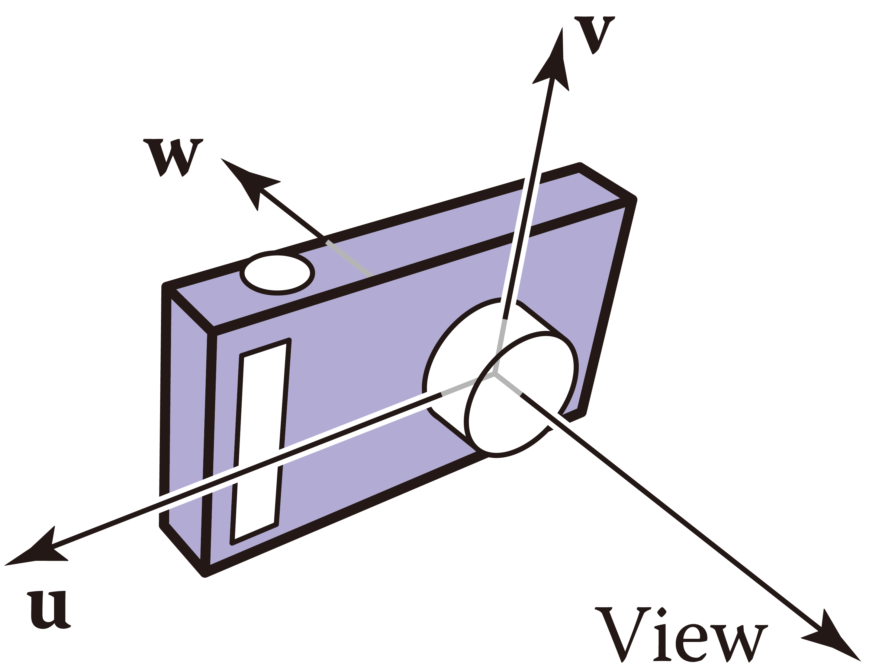
Suppose world frame (canonical coordinates) is characterized by an orthonormal basis $\{\boldsymbol{x}, \boldsymbol{y}, \boldsymbol{z}\}$ and an origin $\boldsymbol{o}$, and that camera space is defined by an orthonormal basis $\{\boldsymbol{u}, \boldsymbol{v}, \boldsymbol{w}\}$ and an origin $\boldsymbol{e}$. Denote camera space parameters w.r.t. canonical coordinates as

$$\begin{bmatrix} \boldsymbol{u}_{\gray{xyz}} & \boldsymbol{v}_{\gray{xyz}} & \boldsymbol{w}_{\gray{xyz}} & \boldsymbol{e}_{\gray{xyz}} \end{bmatrix} = \begin{bmatrix} x_u & x_v & x_w & x_e \\ y_u & y_v & y_w & y_e \\ z_u & z_v & z_w & z_e \end{bmatrix}$$

then p $= \begin{bmatrix}\boldsymbol{u} & \boldsymbol{v} & \boldsymbol{w} & \boldsymbol{e}\end{bmatrix} \in \mathbb{R}^{3 \times 4}$ is the frame-to-canonical matrix that maps rays in camera space to world coordinates

def get_rays_np(H, W, K, c2w):
    i, j = np.meshgrid(np.arange(W, dtype=np.float32), np.arange(H, dtype=np.float32), indexing='xy')
    dirs = np.stack([ (i-K[0][2]) / K[0][0],
                     -(j-K[1][2]) / K[1][1],
                     -np.ones_like(i)       ], -1)
    # rotate ray directions from camera frame to the world frame
    rays_d = np.sum(dirs[..., np.newaxis, :] * c2w[:3,:3], -1)  # dot product, equals to: [c2w.dot(dir) for dir in dirs]
    # translate camera frame's origin to the world frame. It is the origin of all rays.
    rays_o = np.broadcast_to(c2w[:3,-1], np.shape(rays_d))
    return rays_o, rays_d

np.meshgrid(…) at line $\verb|2|$ creates a 2D grid of points $[0, H) \times [0, W)$, where arrays i and j are respectively the $x$- and $y$ coordinates of the grid points. However, the image plane is bounded by

$$\begin{align*} \text{\blue{b}ottom: } v &= -\frac{H}{2} \\ \text{\blue{t}op: } v &= -\frac{H}{2} \\ \text{\blue{l}eft: } u &= -\frac{W}{2} \\ \text{\blue{r}ight: } u &= \frac{W}{2} \end{align*}$$

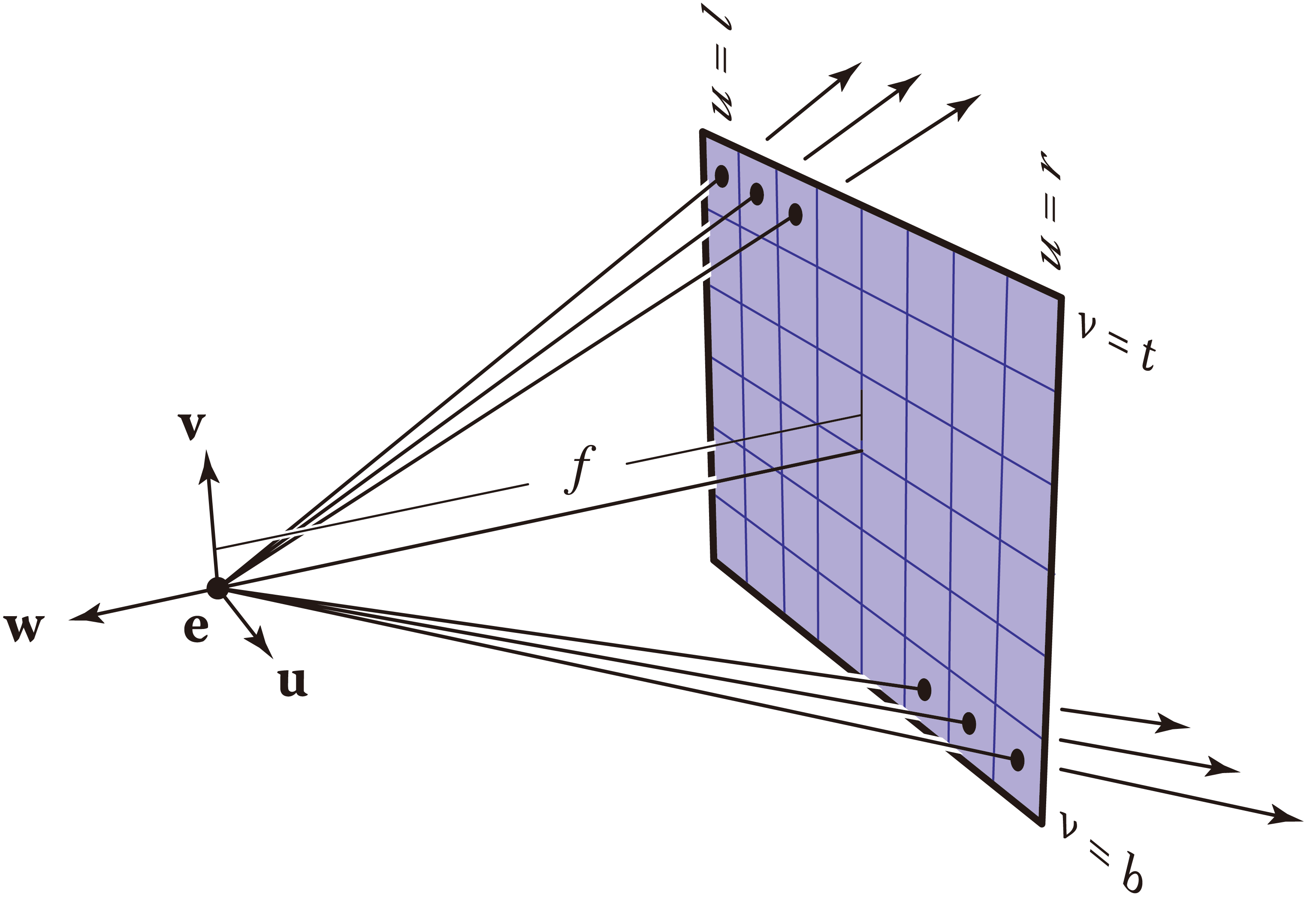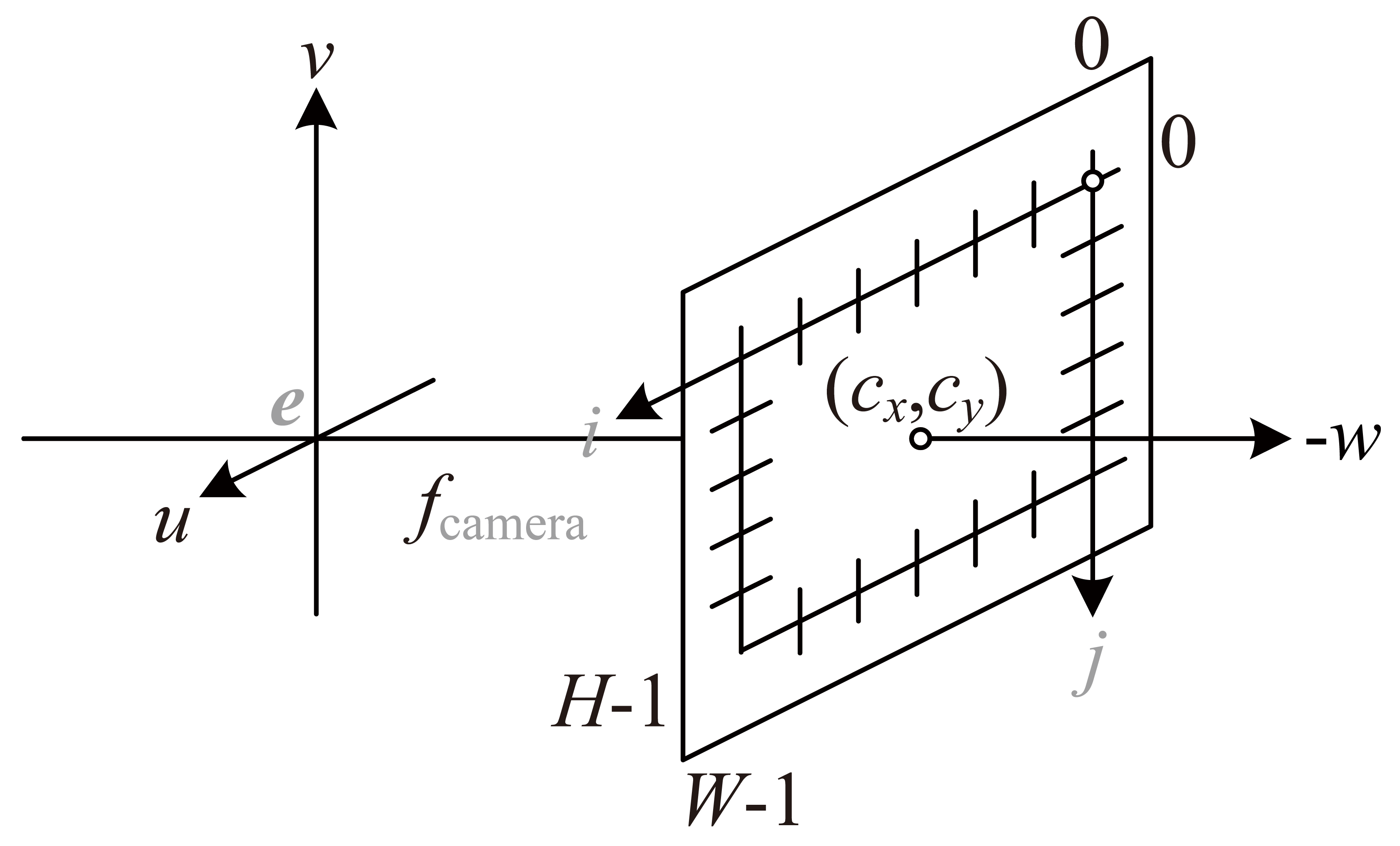Applying an offset, pixel coordinates are $\begin{bmatrix} i - \frac{W}{2} & j - \frac{H}{2} & -f_\text{camera} \end{bmatrix}^\mathsf{T}$ in camera frame. A ray is defined by an origin $\boldsymbol{o}_\text{ray}$, which lies at the origin $\boldsymbol{e}$, and its direction $\boldsymbol{d}$ that connects the origin to a pixel. For every pixel $\boldsymbol{p}$ on the image plane, an ejective direction is

$$\begin{align*} \boldsymbol{d} &= \boldsymbol{p} - \boldsymbol{o}_\text{ray} \\ &= \begin{bmatrix} i - \frac{W}{2} \\ j - \frac{H}{2} \\ -f_\text{camera} \end{bmatrix} \gray{- \boldsymbol{0}} \end{align*}$$

which is then "normalized" to $\hat{\boldsymbol{d}} = \frac{\boldsymbol{d}}{f_\text{camera}} = \begin{bmatrix} \frac{i - W/2}{f_\text{camera}} & \frac{j - H/2}{f_\text{camera}} & -1 \end{bmatrix}^\mathsf{T}$. This corresponds to lines $\verb|3|$ to $\verb|5|$, except that dirs for an entire image are generated concurrently. Note that $j$-axis is opposite to $v$-axis. Consequently, line $\verb|4|$ adopts $-j + \frac{H}{2}$ (instead of $j - \frac{H}{2}$) as $v$-coordinate of $\boldsymbol{d}$.

Rays are then mapped to world space. Apply a linear transformation c2w to directions $\boldsymbol{d}$ to obtain rays_d (line $\verb|7|$) . Ray origins rays_o are simply $\boldsymbol{e}$, the last column of c2w (line $\verb|9|$). It is broadcast to match the dimension of rays_d.

Coordinate transformation

A point $\boldsymbol{p}_{\gray{uvw}} = \begin{bmatrix}u_{\gray{p}} & v_{\gray{p}} & w_{\gray{p}}\end{bmatrix}^\mathsf{T}$ in camera coordinates is characterized by

$$\boldsymbol{p}_{\gray{uvw}} = \gray{\boldsymbol{e}_{xyz} +} u_{\gray{p}}\boldsymbol{u}_{\gray{xyz}} + v_{\gray{p}}\boldsymbol{v}_{\gray{xyz}} + w_{\gray{p}}\boldsymbol{w}_{\gray{xyz}}$$

alternatively, the same point $\boldsymbol{p}_{\gray{xyz}} = \begin{bmatrix}x_{\gray{p}} & y_{\gray{p}} & z_{\gray{p}}\end{bmatrix}^\mathsf{T}$ in world space is

$$\boldsymbol{p}_{\gray{xyz}} = \gray{\boldsymbol{o} +} x_{\gray{p}}\boldsymbol{x} + y_{\gray{p}}\boldsymbol{y} + z_{\gray{p}}\boldsymbol{z}$$

then $\boldsymbol{p}_{\gray{xyz}}$ and $\boldsymbol{p}_{\gray{uvw}}$ are bridged by

$$\begin{align*} \begin{bmatrix} \boldsymbol{p}_{\gray{xyz}} \\ 1 \end{bmatrix} = \begin{bmatrix} x_{\gray{p}} \\ y_{\gray{p}} \\ z_{\gray{p}} \\ 1 \end{bmatrix} &= \underbrace{\begin{bmatrix} \mathbf{I}_{3 \times 3} & \begin{matrix} x_e \\ y_e \\ z_e \end{matrix} \\ \boldsymbol{0}_{1 \times 3} & 1 \end{bmatrix}}_\text{translation: origins coincide} \underbrace{\begin{bmatrix} \begin{matrix} x_u & x_v & x_w \\ y_u & y_v & y_w \\ z_u & z_v & z_w \end{matrix} & \boldsymbol{0}_{3 \times 1} \\ \boldsymbol{0}_{1 \times 3} & 1 \end{bmatrix}}_\text{rotation: axes align} \begin{bmatrix} u_{\gray{p}} \\ v_{\gray{p}} \\ w_{\gray{p}} \\ 1 \end{bmatrix} \\ &= \begin{bmatrix} \begin{matrix} x_u & x_v & x_w \\ y_u & y_v & y_w \\ z_u & z_v & z_w \end{matrix} & \begin{matrix} x_e \\ y_e \\ z_e \end{matrix} \\ \boldsymbol{0}_{1 \times 3} & 1 \end{bmatrix} \begin{bmatrix} \boldsymbol{p}_{\gray{uvw}} \\ 1 \end{bmatrix} \\ &= \underbrace{\begin{bmatrix} \begin{matrix} \boldsymbol{u} & \boldsymbol{v} & \boldsymbol{w} \end{matrix} & \boldsymbol{e} \\ \boldsymbol{0}_{1 \times 3} & 1 \end{bmatrix}}_\text{frame-to-canonical matrix} \begin{bmatrix} \boldsymbol{p}_{\gray{uvw}} \\ 1 \end{bmatrix} \end{align*}$$

Check 3B1B's videos (linear transformation, matrix multiplication, and 3D trnsformation) on linear algebra to comprehend what the above linear transformations (matrices) physically mean.

The returned values are

Variable	Type	Dimension	Description
rays_o	NumPy array	$(H, W, 3)$	directions of rays in the image plane
rays_d	NumPy array	$(H, W, 3)$	origins of rays in the image plane

Training preparation

def train_prepare(self, data):
    …
    # move training data to GPU
    if use_batching:
        images = torch.Tensor(images).to(device)
    poses = torch.Tensor(poses).to(device)
    if use_batching:
        rays_rgb = torch.Tensor(rays_rgb).to(device)


    N_iters = 200000 + 1
    print('Begin')
    print('TRAIN views are', i_train)
    print('TEST views are', i_test)
    print('VAL views are', i_val)

    # summary writers
    #writer = SummaryWriter(os.path.join(basedir, 'summaries', expname))
    
    start = start + 1
    for i in trange(start, N_iters):
        time0 = time.time()

        # sample random ray batch
        if use_batching:
            # random over all images
            batch = rays_rgb[i_batch:i_batch+N_rand] # [B, 2+1, 3*?]
            batch = torch.transpose(batch, 0, 1)
            batch_rays, target_s = batch[:2], batch[2]

            i_batch += N_rand
            if i_batch >= rays_rgb.shape[0]:
                print("Shuffle data after an epoch!")
                rand_idx = torch.randperm(rays_rgb.shape[0])
                rays_rgb = rays_rgb[rand_idx]
                i_batch = 0
        else:
            …

Lines $\verb|2|$ to $\verb|6|$ convert the training set (from NumPy arrays) to PyTorch tensors and "transfer" them to GPU RAM, and start = start + 1 (line $\verb|18|$) marks the commencement of training iterations. Training data were first divided into batches. Let $B$ denote the batch size ($B =$ N_rand), then inputs batch_rays and ground truth target_s have shape $(2, B, 3)$ and $(B, 3)$ (line $\verb|27|$). Lines $\verb|30|$ to $\verb|34|$ handles out-of-bound cases where the index i_batch exceeds $\verb|num_ray|$. We do not care about the else block starting from line $\verb|35|$ since use_batching is asserted by default.

Rendering

    …
    for i in trange(start, N_iters):
        …
        #####  core optimization loop  #####
        rgb, disp, acc, extras = render(H, W, K, chunk=args.chunk, rays=batch_rays,
                                                 verbose=i < 10, retraw=True,
                                                 **render_kwargs_train)
        …

Ensuing is volume rendering. CL arg chunk defines the number of rays concurrently processed, which impacts performance rather than correctness. render_kwargs_train is a dictionary returned upon initiating a NeRF network (line $\verb|107|$ in train) with $2$ more keys injected at line $\verb|112|$ (in train). Its internals are

Key	Element	Description
network_query_fn	a function	a subroutine that takes data and a network as input to perform query
perturb	1.	whether to adopt stratified sampling, 1. for True
N_importance	$128$	number of addition samples $N_F$ per ray in hierarchical sampling
network_fine	an object	the fine network
N_samples	$64$	number of samples $N_C$ per ray to coarse network
network_fn	an object	the coarse network
use_viewdirs	True	whether to feed viewing directions to network, indispensible for view-dependent apprearance
white_bkgd	False	whether to assume white background for rendering This applies to the synthetic dataset only, which contains images (.png) with transparent background.
raw_noise_std	1.	magnitude of noise to inject into volume density
near	0.	lower bound of rendering integration
far	1.	upper bound of rendering integration

Note

See appendix for how a NeRF model is implemented.

Basic procedure

def render(H, W, K, chunk=1024*32, rays=None, c2w=None, ndc=True,
           near=0., far=1.,
           use_viewdirs=False, c2w_staticcam=None,
           **kwargs):
    if c2w is not None:
        # special case to render full image
        rays_o, rays_d = get_rays(H, W, K, c2w)
    else:
        # use provided ray batch
        rays_o, rays_d = rays
    # provide ray directions as input
    if use_viewdirs:
        viewdirs = rays_d
        if c2w_staticcam is not None:
            # special case to visualize effect of viewdirs
            rays_o, rays_d = get_rays(H, W, K, c2w_staticcam)
        viewdirs = viewdirs / torch.norm(viewdirs, dim=-1, keepdim=True)
        viewdirs = torch.reshape(viewdirs, [-1,3]).float()

    sh = rays_d.shape # shape: … × 3
    # for forward facing scenes
    if ndc:
        rays_o, rays_d = ndc_rays(H, W, K[0][0], 1., rays_o, rays_d)
    # create ray batch
    rays_o = torch.reshape(rays_o, [-1,3]).float()
    rays_d = torch.reshape(rays_d, [-1,3]).float()
    near, far = near * torch.ones_like(rays_d[...,:1]), \
                far  * torch.ones_like(rays_d[...,:1])
    rays = torch.cat([rays_o, rays_d, near, far], -1)
    if use_viewdirs:
        rays = torch.cat([rays, viewdirs], -1)
    # render and reshape
    all_ret = batchify_rays(rays, chunk, **kwargs)
    for k in all_ret:
        k_sh = list(sh[:-1]) + list(all_ret[k].shape[1:])
        all_ret[k] = torch.reshape(all_ret[k], k_sh)

    k_extract = ['rgb_map', 'disp_map', 'acc_map']
    ret_list = [all_ret[k] for k in k_extract]
    ret_dict = {k : all_ret[k] for k in all_ret
                                   if k not in k_extract}
    return ret_list + [ret_dict]

Lines $\verb|5|$ to $\verb|7|$ and $\verb|14|$ to $\verb|16|$ are ignored because the conditions contradict the default setting. Rays are unpacked to origins and directions at line $\verb|10|$. Viewing directions are aliases to ray directions (line $\verb|13|$) except that they are normalized at line $\verb|17|$. Rays are then projected to NDC space at line $\verb|23|$; see my other post for details. near $= \mathbf{O}_{B \times 3}$ and far $= \mathbf{J}_{B \times 3}$ are initiated (lines $\verb|27|$ and $\verb|28|$) to match the shape of rays_d. All the above are concatenated (lines $\verb|29|$ to $\verb|31|$) such that input to the network rays have dimension $(B, \gray{\verb|rays_o|:} 3 + \gray{\verb|rays_d|:} 3 + \gray{\verb|near|:} 1 + \gray{\verb|far|:} 1 + \gray{\verb|viewdirs|:} 3) = (B, 11)$.

batchify_rays(…) at line $\verb|33|$ (see right tab) decomposes the input tensor into mini-batches to feed to the NeRF network sequentially. There are $8$ elements in the all_ret dictionary at line $\verb|36|$:

Key	Description of element
rgb_map	output color map of the fine network
disp_map	output disparity map of the fine network
acc_map	output accumulated transmittance of the fine network
raw	raw output of the fine network
rgb0	output color map of the coarse network
disp0	output disparity map of the coarse network
acc0	output accumulated transmittance of the coarse network
z_std	standard variance of disparities of samples along each ray

The ensuing lines (line $\verb|38|$ onward) group and reorder the output such that what are returned can be properly unpacked by train(…)

Mini-batch operation

def batchify_rays(rays_flat, chunk=1024*32, **kwargs):
    """ render rays in smaller minibatches to avoid OOM
    """
    all_ret = {}
    for i in range(0, rays_flat.shape[0], chunk):
        ret = render_rays(rays_flat[i:i+chunk], **kwargs)
        for k in ret:
            if k not in all_ret:
                all_ret[k] = []
            all_ret[k].append(ret[k])
    all_ret = {k : torch.cat(all_ret[k], 0) for k in all_ret}

    return all_ret

Mini-batches are sequentially passed to render_rays(…) (see below) at line $\verb|6|$, cached from line $\verb|7|$ to $\verb|10|$, and eventually concatenated at line $\verb|11|$. We may consider batchify_rays(…) as a broker connecting the high-level interface (render(…)) to actual rendering implementation.

Keyword arguments are passed from high-level interface to "worker" procedures.

By encapsulation with batchify_rays(…) and render(…), training options render_kwargs_train defined previously are passed to the low-level "worker" render_rays(…), which is to core of volume rendering.

Rendering each ray

def render_rays(ray_batch,
                network_fn,
                network_query_fn,
                N_samples,
                retraw=False,
                lindisp=False,
                perturb=0., # 1.0, overridden by input
                N_importance=0,
                network_fine=None,
                white_bkgd=False,
                raw_noise_std=0.,
                verbose=False,
                pytest=False):
    N_rays = ray_batch.shape[0]
    rays_o, rays_d = ray_batch[:,0:3], \
                     ray_batch[:,3:6] # (ray #, 3)
    viewdirs = ray_batch[:,-3:] if ray_batch.shape[-1] > 8 \
                                else None
    bounds = torch.reshape(ray_batch[...,6:8], [-1,1,2])
    near, far = bounds[...,0], \
                bounds[...,1] # (ray #, 1)
    t_vals = torch.linspace(0., 1., steps=N_samples)
    if not lindisp:
        z_vals = near * (1. - t_vals) + far * t_vals
    else:
        z_vals = 1. / (1./near * (1. - t_vals) +
                       1./far  * (     t_vals) )
    # copy sample distances of 1 ray to the others
    z_vals = z_vals.expand([N_rays, N_samples])

    if perturb > 0.:
        # get intervals between samples
        mids = .5 * (z_vals[...,1:] + z_vals[...,:-1])
        upper = torch.cat([mids, z_vals[...,-1:]], -1)
        lower = torch.cat([z_vals[...,:1], mids], -1)
        # stratified samples in those intervals
        t_rand = torch.rand(z_vals.shape)
        # pytest: overwrite U with fixed NumPy random numbers
        if pytest:
            np.random.seed(0)
            t_rand = np.random.rand(*list(z_vals.shape))
            t_rand = torch.Tensor(t_rand)

        z_vals = lower + (upper - lower) * t_rand

    pts = rays_o[..., None, :] + \
          rays_d[..., None, :] * z_vals[..., :, None] # (ray #, sample #, 3)
    #raw = run_network(pts)
    raw = network_query_fn(pts, viewdirs, network_fn)
    rgb_map, disp_map, acc_map, weights, depth_map = raw2outputs(raw, z_vals, rays_d, raw_noise_std, white_bkgd, pytest=pytest)
    # hierarchical sampling
    if N_importance > 0:
        # log outputs of coarse network
        rgb_map_0, disp_map_0, acc_map_0 = rgb_map, disp_map, acc_map

        z_vals_mid = .5 * (z_vals[..., 1: ] + z_vals[..., :-1])
        z_samples = sample_pdf(z_vals_mid,
                               weights[..., 1:-1],
                               N_importance,
                               det=(perturb==0.), # FALSE by default
                               pytest=pytest)
        z_samples = z_samples.detach()

        z_vals, _ = torch.sort(torch.cat([z_vals, z_samples], -1), -1)
        pts = rays_o[..., None, :] + \
              rays_d[..., None, :] * z_vals[..., :, None] # (ray #, coarse & fine sample #, 3)

        run_fn = network_fn if   network_fine is None \
                            else network_fine
        #raw = run_network(pts, fn=run_fn)
        raw = network_query_fn(pts, viewdirs, run_fn)

        rgb_map, disp_map, acc_map, weights, depth_map = raw2outputs(raw, z_vals, rays_d, raw_noise_std, white_bkgd, pytest=pytest)

    ret = {'rgb_map' :  rgb_map,
           'disp_map': disp_map,
           'acc_map' :  acc_map}
    if retraw:
        ret['raw'] = raw
    if N_importance > 0:
        ret['rgb0' ] =  rgb_map_0
        ret['disp0'] = disp_map_0
        ret['acc0' ] =  acc_map_0
        ret['z_std'] = torch.std(z_samples, dim=-1, unbiased=False)  # (ray #)
    for k in ret:
        if (torch.isnan(ret[k]).any() or torch.isinf(ret[k]).any()) and DEBUG:
            print(f"! [Numerical Error] {k} contains nan or inf.")
    return ret

Lines $\verb|14|$ to $\verb|21|$ unpack each mini-batch to separate physical values. Ray origins rays_o, ray directions rays_d, and viewing directions viewdirs have shape $(B, 3)$. Integration boundaries near and far are both $B \times 1$ vectors.

Lines $\verb|22|$ to $\verb|44|$ initialize the samples for ray marching. torch.linspace(…) at line $\verb|22|$ create a sequence of $N_C$ points evenly scattered along unit length. Recall that rays are previously projected to NDC space. False by default, lindisp dictates the voxels are sampled linearly on disparity (inverse depth). z_vals simply replicates t_vals (lines $\verb|24|$ and $\verb|29|$) to modulate all points on a batch of rays.

There are $N_C - 1$ intervals along each ray. To pick $N_C$ random points out of those intervals ("bins"), at least $2$ of them should have length less than $\frac{1}{N_C - 1}$. The authors cut the first and last "bin" in half so that all $N_C$ "bins" fit to the interval $[0, 1]$. Line $\verb|33|$ determines of midpoints of z_vals, which are afterwards combined with the start (line $\verb|35|$) and endpoint bound (line $\verb|34|$) of each ray.

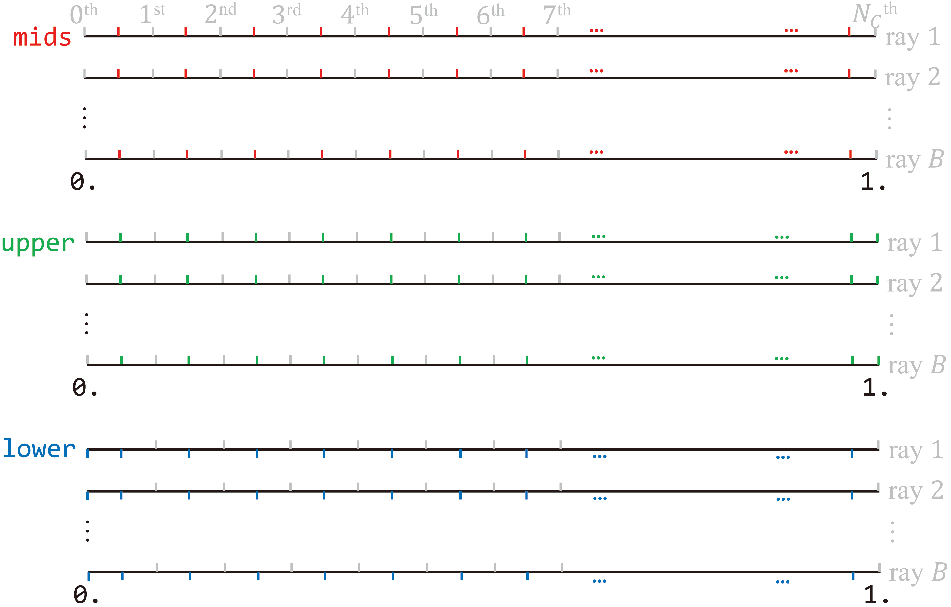
Subtracting the lower bound from the upper bound finalizes the length of "bins", and stratified sampling is achieved by uniformly sampling every interval. Now, sample $z_i$ lies in bin $i \ \forall i \in \{1, 2, \ldots, N_C\}$.

Let $z_i^{(b)}$ denote the $i$^th sample on the $b$^th ray in a batch, then z_vals at line $\verb|44|$ is

$$\verb|z_vals| = \begin{bmatrix} z_1^{(1)} & z_2^{(1)} & \cdots & z_{N_C}^{(1)} \\ z_1^{(2)} & z_2^{(2)} & \cdots & z_{N_C}^{(2)} \\ \vdots & \vdots & \ddots & \vdots \\ z_1^{(B)} & z_2^{(B)} & \cdots & z_{N_C}^{(B)} \end{bmatrix}$$

Sampling: slight deviation of practice from theory

Implementation of stratified sampling is inconsistent with what is described in the paper. Theoretically, a sample $z_i$ is obtained via

$$t_i \sim \mathcal{U}\left[ \verb|near| + \frac{i-1}{N_C} (\verb|far| - \verb|near|), \verb|near| + \frac{i}{N_C} (\verb|far| - \verb|near|) \right]$$

which implies each "bin" is of equal length. The first and last bins, in practice, are half the size of the others. This does not harm the correctness of the algorithm.

Marching depth values z_vals along directions rays_d, inputs pts to network_fn at lines $\verb|46|$ and $\verb|47|$ are now

$$\boldsymbol{r}_{\gray{B \times N_C \times 3}} = \begin{bmatrix} \boldsymbol{e}^{(1)} + z_1^{(1)} \boldsymbol{d}^{(1)} & \boldsymbol{e}^{(1)} + z_2^{(1)} \boldsymbol{d}^{(1)} & \cdots & \boldsymbol{e}^{(1)} + z_{N_C}^{(1)} \boldsymbol{d}^{(1)} \\ \boldsymbol{e}^{(2)} + z_1^{(2)} \boldsymbol{d}^{(2)} & \boldsymbol{e}^{(2)} + z_2^{(2)} \boldsymbol{d}^{(2)} & \cdots & \boldsymbol{e}^{(2)} + z_{N_C}^{(2)} \boldsymbol{d}^{(2)} \\ \vdots & \vdots & \ddots & \vdots \\ \boldsymbol{e}^{(B)} + z_1^{(B)} \boldsymbol{d}^{(B)} & \boldsymbol{e}^{(B)} + z_2^{(B)} \boldsymbol{d}^{(B)} & \cdots & \boldsymbol{e}^{(B)} + z_{N_C}^{(B)} \boldsymbol{d}^{(B)} \end{bmatrix}$$

The coarse network network_fn is then queried at line $\verb|49|$ to predict raw output raw (see appendix for how NeRF is queried). raw has shape $(B, \gray{\verb|rgb|:} 3 + \gray{\sigma:} 1) = (B, 4)$. "Shading" via raw2outputs(…) follows at line $\verb|50|$ to acquire sample weights and radiance of each ray (see middle tab).

To distinguish outputs of the fine network from those of the coarse one, prefixes _0 are appended to initial outputs at line $\verb|54|$. Provided z_vals_mid, midpoints of coarse samples (line $\verb|56|$) and their weights $\mathbf{W}_{\gray{B \times N_C}}$, lines $\verb|57|$ to $\verb|61|$ determine fine samples (see right tab). They are combined with coarse samples at line $\verb|64|$ to form a sorted tensor of disparities z_vals

$$\verb|z_vals| = \begin{bmatrix} z_1^{(1)} & z_2^{(1)} & \cdots & z_{N_C \blue{+ N_F}}^{(1)} \\ z_1^{(2)} & z_2^{(2)} & \cdots & z_{N_C \blue{+ N_F}}^{(2)} \\ \vdots & \vdots & \ddots & \vdots \\ z_1^{(B)} & z_2^{(B)} & \cdots & z_{N_C \blue{+ N_F}}^{(B)} \end{bmatrix}$$

Static compute graph

NeRF spans a static computate graph. The key is the ….detach() call at line $\verb|62|$.

The coarse-to-fine passes are connected by hierarchical sampling, i.e., output of the coarse MLP is used to determine the input of the fine network. Bellow illustrates how the coarse samples are processed to for the fine ones:

$$\left. \begin{array}{r} \left. \begin{array}{r} \left. \begin{array}{r} \green{\verb|z_vals|_\text{coarse}} \xrightarrow[\text{lines \texttt{46} and \texttt{47}}]{} \verb|pts| \\ \cdots \end{array} \right\} \xrightarrow[\text{line \texttt{49}}]{\red{\verb|network_query_fn|}} \verb|raw| \xrightarrow[\text{line \texttt{50}}]{\verb|raw2outputs|} \cdots,~\verb|weights| \\ \green{\verb|z_vals|_\text{coarse}} \xrightarrow[\text{line \texttt{56}}]{} \verb|z_vals_mid| \\ \cdots \end{array} \right\} \xrightarrow[\text{lines \texttt{57} to \texttt{61}}]{\verb|sample_pdf|} \verb|z_samples| \\ \verb|z_vals| \end{array} \right\} \xrightarrow[\text{line \texttt{64}}]{\text{concatenation}} ~ \xrightarrow[\text{line \texttt{64}}]{\text{sorting}} \blue{\verb|z_vals|_\text{fine}}$$

Hierarchically sampled inputs are again fed to the network.

$$\left. \begin{array}{r} \blue{\verb|z_vals|_\text{fine}} \xrightarrow[\text{lines \texttt{65} and \texttt{66}}]{} \verb|pts| \\ \cdots \end{array} \right\} \xrightarrow[\text{line \texttt{71}}]{\red{\verb|network_query_fn|}} \cdots$$

Consequently, output of the MLP becomes part of its input. It is a must to cut the coarse-to-fine edge in the compute graph because it has to be a directed acyclic one. Otherwise, if the fine network shared with the coarse one an identical instance of class NeRF, there would be cyclic definition, and backpropagation would fail. This is exactly what z_samples.detach() does at line $\verb|62|$.

A corollary is that NeRF's compute graph is static.

New inputs pts to the fine network network_fine at lines $\verb|65|$ and $\verb|66|$ are now

$$\boldsymbol{r}_{\gray{B \times N_C \times 3}} = \begin{bmatrix} \boldsymbol{e}^{(1)} + z_1^{(1)} \boldsymbol{d}^{(1)} & \boldsymbol{e}^{(1)} + z_2^{(1)} \boldsymbol{d}^{(1)} & \cdots & \boldsymbol{e}^{(1)} + z_{N_C \blue{+ N_F}}^{(1)} \boldsymbol{d}^{(1)} \\ \boldsymbol{e}^{(2)} + z_1^{(2)} \boldsymbol{d}^{(2)} & \boldsymbol{e}^{(2)} + z_2^{(2)} \boldsymbol{d}^{(2)} & \cdots & \boldsymbol{e}^{(2)} + z_{N_C \blue{+ N_F}}^{(2)} \boldsymbol{d}^{(2)} \\ \vdots & \vdots & \ddots & \vdots \\ \boldsymbol{e}^{(B)} + z_1^{(B)} \boldsymbol{d}^{(B)} & \boldsymbol{e}^{(B)} + z_2^{(B)} \boldsymbol{d}^{(B)} & \cdots & \boldsymbol{e}^{(B)} + z_{N_C \blue{+ N_F}}^{(B)} \boldsymbol{d}^{(B)} \end{bmatrix}$$

Another mass network query is performed at line $\verb|71|$, whose raw outputs are converted to radiance rgb_map at $\verb|71|$.

Shading

def raw2outputs(raw, z_vals, rays_d, raw_noise_std=0, white_bkgd=False, pytest=False):
    raw2alpha = lambda raw, dists, act_fn=F.relu : \
                       1. - torch.exp(-act_fn(raw) * dists) # σ column of `raw`

    dists = z_vals[..., 1:] - z_vals[..., :-1]
    dists = torch.cat([dists, # (ray #, sample #)
                       torch.Tensor([1e10]).expand(dists[..., :1].shape)],
                       -1)
    dists = dists * torch.norm(rays_d[..., None, :], dim=-1)

    rgb = torch.sigmoid(raw[..., :3]) # (ray #, sample #, 3)

    noise = 0.
    if raw_noise_std > 0.:
        noise = torch.randn(raw[..., 3].shape) * raw_noise_std
        # overwrite randomly sampled data
        if pytest:
            np.random.seed(0)
            noise = np.random.rand(*list(raw[...,3].shape)) * raw_noise_std
            noise = torch.Tensor(noise)

    alpha = raw2alpha(raw[..., 3] + noise, dists) # (ray #, sample #)
    #weights = alpha * tf.math.cumprod(1.-alpha + 1e-10, -1, exclusive=True)
    weights = alpha * torch.cumprod(torch.cat([torch.ones((alpha.shape[0], 1)),
                                               1. - alpha + 1e-10], -1), 
                                    -1)[:, :-1]

    rgb_map   = torch.sum(weights[..., None] * rgb, -2)  # (ray #, 3)
    depth_map = torch.sum(weights * z_vals, -1)
    disp_map  = 1. / torch.max(1e-10 * torch.ones_like(depth_map),
                               depth_map / torch.sum(weights, -1))
    acc_map   = torch.sum(weights, -1)
    if white_bkgd:
        rgb_map = rgb_map + (1. - acc_map[..., None])

    return rgb_map, disp_map, acc_map, weights, depth_map

dists from line $\verb|5|$ to $\verb|9|$ calculates the difference between disparities $\delta_i := z_{i+1} - z_i$.

$$\begin{align*} \mathbf{\Delta}_{\gray{B \times N_C}} &= \begin{bmatrix} \delta_1^{(1)} & \delta_2^{(1)} & \cdots & \delta_{N_C \blue{- 1}}^{(1)} & \gray{\infty} \\ \delta_1^{(2)} & \delta_2^{(2)} & \cdots & \delta_{N_C \blue{- 1}}^{(2)} & \gray{\infty} \\ \vdots & \vdots & \ddots & \vdots & \gray{\vdots} \\ \delta_1^{(B)} & \delta_2^{(B)} & \cdots & \delta_{N_C \blue{- 1}}^{(B)} & \gray{\infty} \\ \end{bmatrix} \\ &= \begin{bmatrix} z_2^{(1)} - z_1^{(1)} & z_3^{(1)} - z_2^{(1)} & \cdots & z_{N_C}^{(1)} - z_{N_C - 1}^{(1)} & \gray{\infty} \\ z_2^{(2)} - z_1^{(2)} & z_3^{(2)} - z_2^{(2)} & \cdots & z_{N_C}^{(2)} - z_{N_C - 1}^{(2)} & \gray{\infty} \\ \vdots & \vdots & \ddots & \vdots & \gray{\vdots} \\ z_2^{(B)} - z_1^{(B)} & z_3^{(B)} - z_2^{(B)} & \cdots & z_{N_C}^{(B)} - z_{N_C - 1}^{(B)} & \gray{\infty} \\ \end{bmatrix} \end{align*}$$

Purpose of appending a large vector

$\verb|1e10| = 10^{10} \approx \infty$ is appended to the last column of $\mathbf{\Delta}_{\gray{B \times N_C}}$ to (a) maintain the shape of dists as $(B, N_C)$, and (b) to force the last column of "opacticy" alpha $\mathbf{\Delta}_{\gray{B \times N_C}}$ to be 1 such that classic alpha compositing holds.

Line $\verb|11|$ forces RGB values rgb to lie in the range $(0, 1)$, that is,

$$\mathbf{c}_{\gray{B \times N_C \times 3}} = \begin{bmatrix} \boldsymbol{c}_1^{(1)} & \boldsymbol{c}_2^{(1)} & \cdots & \boldsymbol{c}_{N_C}^{(1)} \\ \boldsymbol{c}_1^{(2)} & \boldsymbol{c}_2^{(2)} & \cdots & \boldsymbol{c}_{N_C}^{(2)} \\ \vdots & \vdots & \ddots & \vdots \\ \boldsymbol{c}_1^{(B)} & \boldsymbol{c}_2^{(B)} & \cdots & \boldsymbol{c}_{N_C}^{(B)} \\ \end{bmatrix} \forall \boldsymbol{c}_i^{(b)} \in (0, 1)$$

Random noise (line $\verb|15|$) is injected to volume density $\sigma_i^{(b)}$ (line $\verb|15|$) before it is rectified and raised to $\alpha_i^{(b)}$ (lines $\verb|2|$, $\verb|3|$, and $\verb|22|$). Let $\hat{\sigma}_i^{(b)} := \verb|ReLU| \left( \sigma_i^{(b)} + \mathcal{U}[0, 1] \right)$ denote the recitified "opacity" of the $i$^th sample along the $b$^th ray, then alpha for alpha compositing are

$$\begin{align*} \mathbf{\Alpha}_{\gray{B \times N_C}} &= \boldsymbol{1}_{\gray{B \times N_C}} - \exp \left( \boldsymbol{\sigma}_{\gray{B \times N_C}} * \mathbf{\Delta}_{\gray{B \times N_C}} \right) \\ &= \begin{bmatrix} 1 - e^{- \sigma_1^{(1)} \delta_1^{(1)}} & 1 - e^{- \sigma_2^{(1)} \delta_2^{(1)}} & \cdots & 1 - e^{- \sigma_{N_C \blue{- 1}}^{(1)} \delta_{N_C \blue{- 1}}^{(1)}} & 1 \gray{- e^{-\infty}} \\ 1 - e^{- \sigma_1^{(2)} \delta_1^{(2)}} & 1 - e^{- \sigma_2^{(2)} \delta_2^{(2)}} & \cdots & 1 - e^{- \sigma_{N_C \blue{- 1}}^{(2)} \delta_{N_C \blue{- 1}}^{(2)}} & 1 \gray{- e^{-\infty}} \\ \vdots & \vdots & \ddots & \vdots & \vdots \\ 1 - e^{- \sigma_1^{(B)} \delta_1^{(B)}} & 1 - e^{- \sigma_2^{(B)} \delta_2^{(B)}} & \cdots & 1 - e^{- \sigma_{N_C \blue{- 1}}^{(B)} \delta_{N_C \blue{- 1}}^{(B)}} & 1 \gray{- e^{-\infty}} \end{bmatrix} \\ &= \begin{bmatrix} \alpha_1^{(1)} & \alpha_2^{(1)} & \cdots & \alpha_{N_C}^{(1)} \\ \alpha_1^{(2)} & \alpha_2^{(2)} & \cdots & \alpha_{N_C}^{(2)} \\ \vdots & \ddots & \vdots & \vdots \\ \alpha_1^{(B)} & \alpha_2^{(B)} & \cdots & \alpha_{N_C}^{(B)} \end{bmatrix} \end{align*}$$

where $*$ denotes the Hadamard product. torch.cumprod(…) from line $\verb|24|$ to $\verb|26|$ calculates the cumulative transmittance

$$\begin{align*} \mathbf{T}_{\gray{B \times (N_C \blue{+ 1})}} &= \verb|cumprod| \left( \begin{bmatrix} \boldsymbol{1}_{\gray{B \times 1}} \left|\ \boldsymbol{1}_{\gray{B \times N_C}} - \mathbf{\Alpha} \right. \end{bmatrix} \right) \\ &= \verb|cumprod| \left( \begin{bmatrix} 1 & e^{- \sigma_1^{(1)} \delta_1^{(1)}} & e^{- \sigma_2^{(1)} \delta_2^{(1)}} & \cdots & e^{- \sigma_{N_C \blue{- 1}}^{(1)} \delta_{N_C \blue{- 1}}^{(1)}} & 0 \\ 1 & e^{- \sigma_1^{(2)} \delta_1^{(2)}} & e^{- \sigma_2^{(2)} \delta_2^{(2)}} & \cdots & e^{- \sigma_{N_C \blue{- 1}}^{(2)} \delta_{N_C \blue{- 1}}^{(2)}} & 0 \\ \vdots & \vdots & \vdots & \ddots & \vdots & \vdots \\ 1 & e^{- \sigma_1^{(B)} \delta_1^{(B)}} & e^{- \sigma_2^{(B)} \delta_2^{(B)}} & \cdots & e^{- \sigma_{N_C \blue{- 1}}^{(B)} \delta_{N_C \blue{- 1}}^{(B)}} & 0 \end{bmatrix} \right) \\ &= \begin{bmatrix} 1 & e^{- \sigma_1^{(1)} \delta_1^{(1)}} & e^{- \sigma_1^{(1)} \delta_1^{(1)} - \sigma_2^{(1)} \delta_2^{(1)}} & \cdots & \exp \left(-\sum_{j=1}^{N_C\blue{-1}} \sigma_j^{(1)} \delta_j^{(1)} \right) & 0 \\ 1 & e^{- \sigma_1^{(2)} \delta_1^{(2)}} & e^{- \sigma_1^{(2)} \delta_1^{(2)} - \sigma_2^{(2)} \delta_2^{(2)}} & \cdots & \exp \left(-\sum_{j=1}^{N_C\blue{-1}} \sigma_j^{(2)} \delta_j^{(2)} \right) & 0 \\ \vdots & \vdots & \vdots & \ddots & \vdots & \vdots \\ 1 & e^{- \sigma_1^{(B)} \delta_1^{(B)}} & e^{- \sigma_1^{(B)} \delta_1^{(B)} - \sigma_2^{(B)} \delta_2^{(B)}} & \cdots & \exp \left(-\sum_{j=1}^{N_C\blue{-1}} \sigma_j^{(B)} \delta_j^{(B)} \right) & 0 \end{bmatrix} \\ &= \begin{bmatrix} T_1^{(1)} & T_2^{(1)} & \cdots & T_{N_C}^{(1)} & \gray{0} \\ T_1^{(2)} & T_2^{(2)} & \cdots & T_{N_C}^{(2)} & \gray{0} \\ \vdots & \vdots & \ddots & \vdots & \gray{\vdots} \\ T_1^{(B)} & T_2^{(B)} & \cdots & T_{N_C}^{(B)} & \gray{0} \\ \end{bmatrix} \end{align*}$$

The last column of $\mathbf{T}$ is discarded to match the shape of $\mathbf{\Alpha}$. Rewriting weights (for points' colors) as $w_i^{(b)} := \alpha_i^{(b)}T_i^{(b)}$, weights is

$$\begin{align*} \mathbf{W}_{\gray{B \times N_C}} &= \mathbf{\Alpha} * \mathbf{T} \\ &= \begin{bmatrix} \alpha_1^{(1)} \gray{T_1^{(1)}} & \alpha_2^{(1)} T_2^{(1)} & \cdots & \gray{\alpha_{N_C}^{(1)}} T_{N_C}^{(1)} \\ \alpha_1^{(2)} \gray{T_1^{(2)}} & \alpha_2^{(2)} T_2^{(2)} & \cdots & \gray{\alpha_{N_C}^{(2)}} T_{N_C}^{(2)} \\ \vdots & \vdots & \ddots & \vdots \\ \alpha_1^{(B)} \gray{T_1^{(B)}} & \alpha_2^{(B)} T_2^{(B)} & \cdots & \gray{\alpha_{N_C}^{(B)}} T_{N_C}^{(B)} \\ \end{bmatrix} \\ &= \begin{bmatrix} w_1^{(1)} & w_2^{(1)} & \cdots & w_{N_C}^{(1)} \\ w_1^{(2)} & w_2^{(2)} & \cdots & w_{N_C}^{(2)} \\ \vdots & \vdots & \ddots & \vdots \\ w_1^{(B)} & w_2^{(B)} & \cdots & w_{N_C}^{(B)} \\ \end{bmatrix} \end{align*}$$

Recall that radiance is a weighted sum of colors of samples along a ray. This corresponds to line $\verb|28|$, and the output rgb_map is

$$\begin{align*} \mathbf{C}_{\gray{B \times 3}} &= \verb|sum|\left(\mathbf{W} * \mathbf{c}\right) \\ &= \begin{bmatrix} w_1^{(1)} \boldsymbol{c}_1^{(1)} + w_2^{(1)} \boldsymbol{c}_2^{(1)} + \cdots + w_{N_C}^{(1)} \boldsymbol{c}_{N_C}^{(1)} \\ w_1^{(2)} \boldsymbol{c}_1^{(2)} + w_2^{(2)} \boldsymbol{c}_2^{(2)} + \cdots + w_{N_C}^{(2)} \boldsymbol{c}_{N_C}^{(2)} \\ \vdots \\ w_1^{(B)} \boldsymbol{c}_1^{(B)} + w_2^{(B)} \boldsymbol{c}_2^{(B)} + \cdots + w_{N_C}^{(B)} \boldsymbol{c}_{N_C}^{(B)} \\ \end{bmatrix} \\ &= \begin{bmatrix} \mathbf{C}^{(1)} \\ \mathbf{C}^{(2)} \\ \vdots \\ \mathbf{C}^{(B)} \end{bmatrix} \end{align*}$$

rgb_map $\mathbf{C}$ and weights $\mathbf{W}$, along with other values, are returned to render_rays(…).

What else are returned?

Content on the way. Stay tuned!

Hierarchical sampling

sample_pdf(…) in run_nerf_helpers.py performs hierarchical sampling via Monte Carlo method. It is invoked by

        …
        z_samples = sample_pdf(z_vals_mid,
                               weights[..., 1:-1],
                               N_importance,
                               det=(perturb==0.), # FALSE by default
                               pytest=pytest)
        …

in render_rays(…), where z_vals_mid is a tensor of midpoints of coarse sample disparities. Note that the leading and trailing columns of weights are excluded from the input such that

$$\mathbf{W}\verb|[..., 1:-1]| = \begin{bmatrix} w_{\blue{2}}^{(1)} & w_3^{(1)} & \cdots & w_{N_C \blue{- 1}}^{(1)} \\ w_{\blue{2}}^{(2)} & w_3^{(2)} & \cdots & w_{N_C \blue{- 1}}^{(2)} \\ \vdots & \vdots & \ddots & \vdots \\ w_{\blue{2}}^{(B)} & w_3^{(B)} & \cdots & w_{N_C \blue{- 1}}^{(B)} \\ \end{bmatrix}$$

def sample_pdf(bins, weights, N_samples, det=False, pytest=False):
    # get PDF
    weights = weights + 1e-5 # prevent NaN
    pdf = weights / torch.sum(weights, -1, keepdim=True)
    cdf = torch.cumsum(pdf, -1)
    cdf = torch.cat([torch.zeros_like(cdf[..., :1]), cdf], -1)  # (ray #, bin #)
    # Here, `N_samples` refers to `N_importance`.
    if det:
        u = torch.linspace(0., 1., steps=N_samples)
        u = u.expand(list(cdf.shape[:-1]) + [N_samples])
    else:
        u = torch.rand(list(cdf.shape[ :-1]) + [N_samples])
    # if pytest, overwrite u with NumPy fixed random numbers
    if pytest:
        np.random.seed(0)
        new_shape = list(cdf.shape[:-1]) + [N_samples]
        if det:
            u = np.linspace(0., 1., N_samples)
            u = np.broadcast_to(u, new_shape)
        else:
            u = np.random.rand(*new_shape)
        u = torch.Tensor(u)
    # invert CDF
    u = u.contiguous()
    inds   = torch.searchsorted(cdf, u, right=True)
    below  = torch.max(torch.zeros_like(inds-1), inds-1)
    above  = torch.min((cdf.shape[-1]-1) * torch.ones_like(inds), inds)
    inds_g = torch.stack([below, above], -1)  # (ray #, sample #, 2)

    #cdf_g  = tf.gather(cdf , inds_g, axis=-1, batch_dims=len(inds_g.shape)-2)
    #bins_g = tf.gather(bins, inds_g, axis=-1, batch_dims=len(inds_g.shape)-2)
    matched_shape = [inds_g.shape[0], inds_g.shape[1], cdf.shape[-1]]
    cdf_g  = torch.gather( cdf.unsqueeze(1).expand(matched_shape), 2, inds_g)
    bins_g = torch.gather(bins.unsqueeze(1).expand(matched_shape), 2, inds_g)

    denom = cdf_g[..., 1] - cdf_g[..., 0]
    denom = torch.where(denom<1e-5, torch.ones_like(denom),
                                    denom)
    t = (u - cdf_g[..., 0]) / denom
    samples =  bins_g[..., 0] + \
              (bins_g[..., 1] - bins_g[..., 0]) * t
    return samples # (ray #, sample #), unsorted along each ray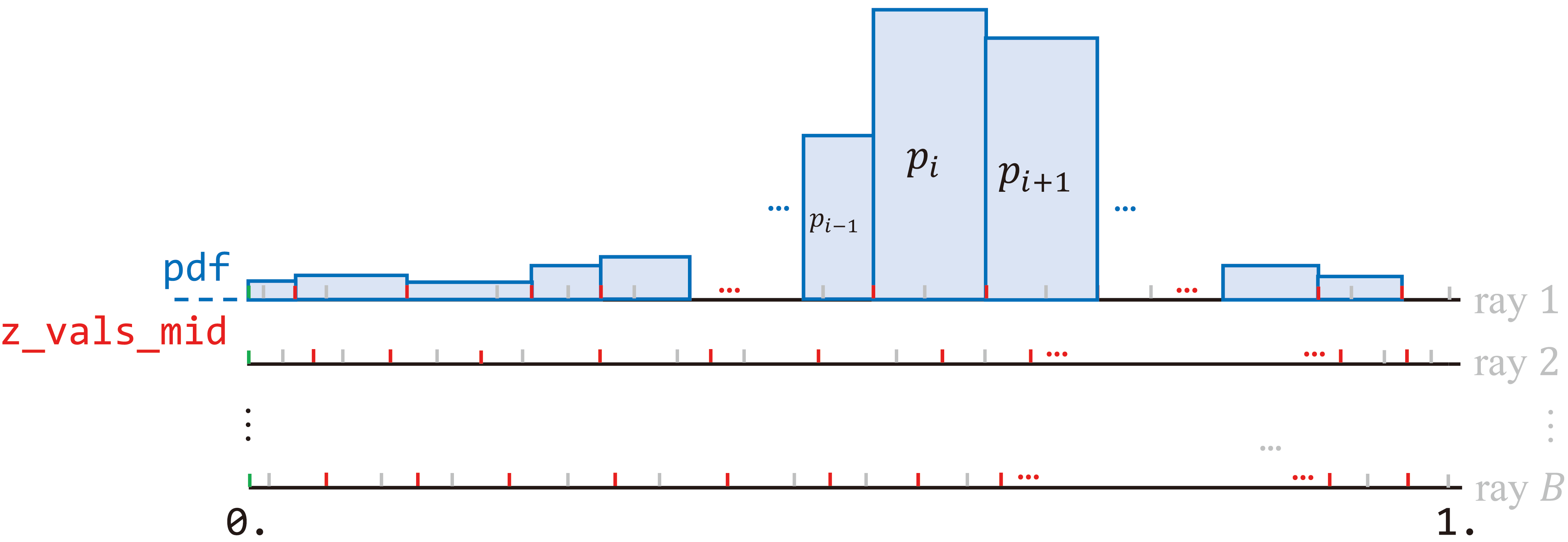

Line $\verb|4|$ defines the probability $p_i$$:= \frac{w_i}{\sum_{j=\blue{2}}^{\blue{N_C-1}} w_j}$ that a ray is stopped by a particle at depth $\frac{z_i + z_{i+1}}{2}$. This corresponds to the area under the histogram, shown above (first ray only).

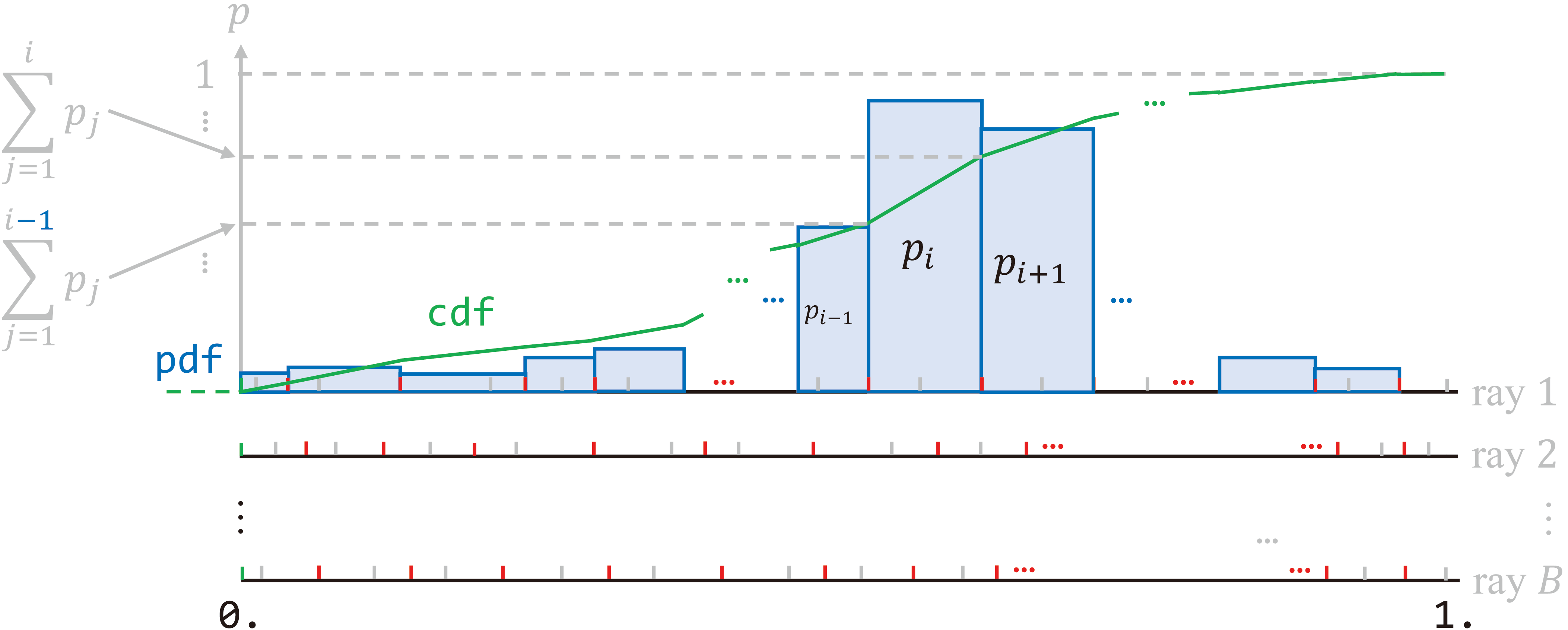
Lines $\verb|5|$ and $\verb|6|$ accumulate the area for the CDF $H(z)$.

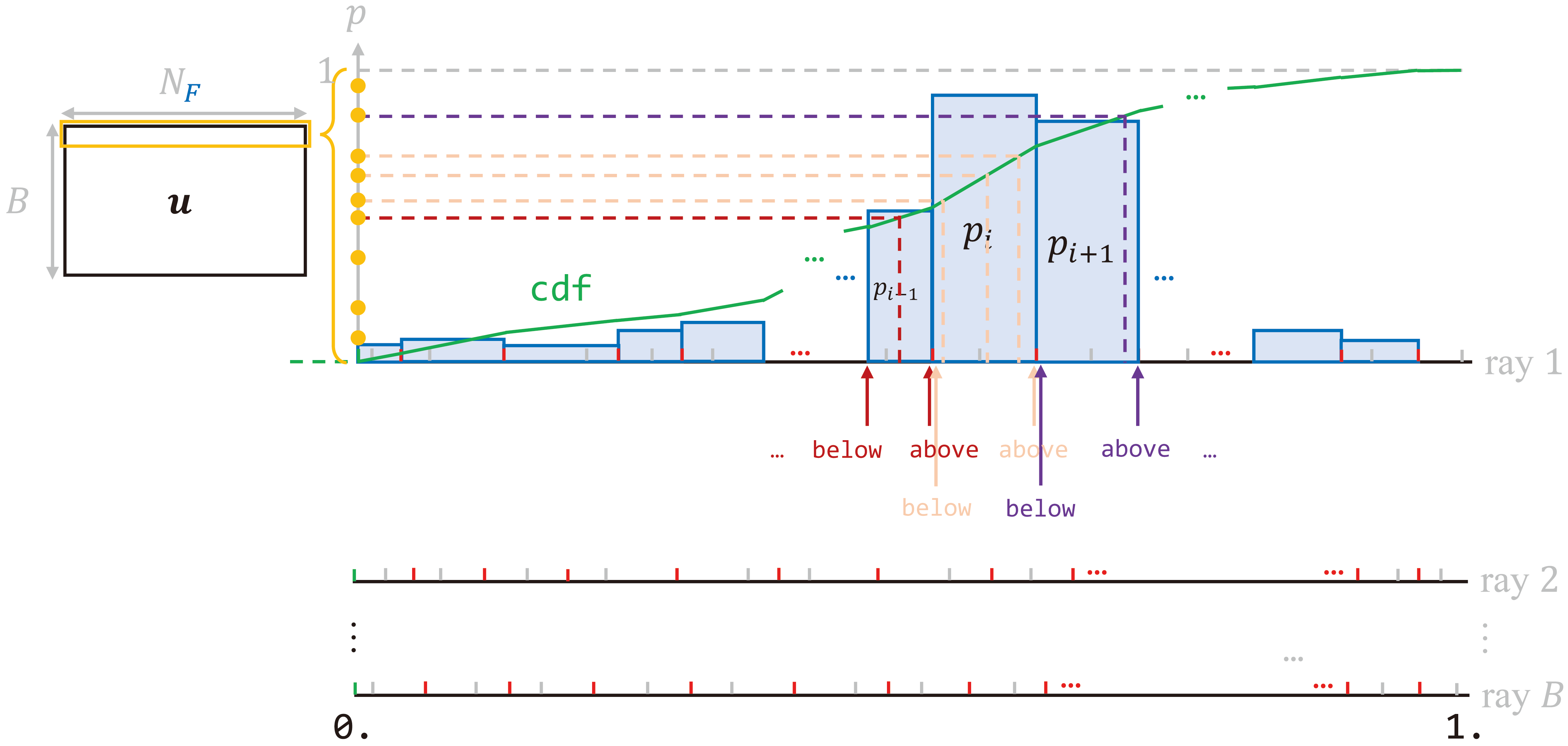
What follows is key to Monte Carlo sampling. Line $\verb|12|$ generates a batch $\mathbf{u}_{\gray{B \times N_F}}$ of random cumulative probabilities — "seeds". The above figure visualizes operations on u[0, :], i.e., $N_F$ seeds on the first ray. They fall into the "bins" at line $\verb|25|$ through comparison against the cumulative probabilities at the boundaries. torch.searchsorted(…) returns the positions (indices) inds $\in \mathbb{R}^{B \times N_F}$ of those random "seeds".

Quicker indicing

torch.Tensor.contiguous() returns a tensor with identical data but contiguous in memory. It is called before torch.searchsorted(…) for performance concern.

Lower bounds of the "bins" are collected as below at line $\verb|26|$, and upper bounds are gathered as above at line $\verb|27|$. inds_g $\in \mathbb{R}^{B \times N_F \times 2}$ combines below and above at line $\verb|28|$. torch.gather(…) at lines $\verb|33|$ and $\verb|34|$ determine how $N_F$ points along each ray are distributed according to indices inds_g, or effectively the number of "seeds" in each "bin".

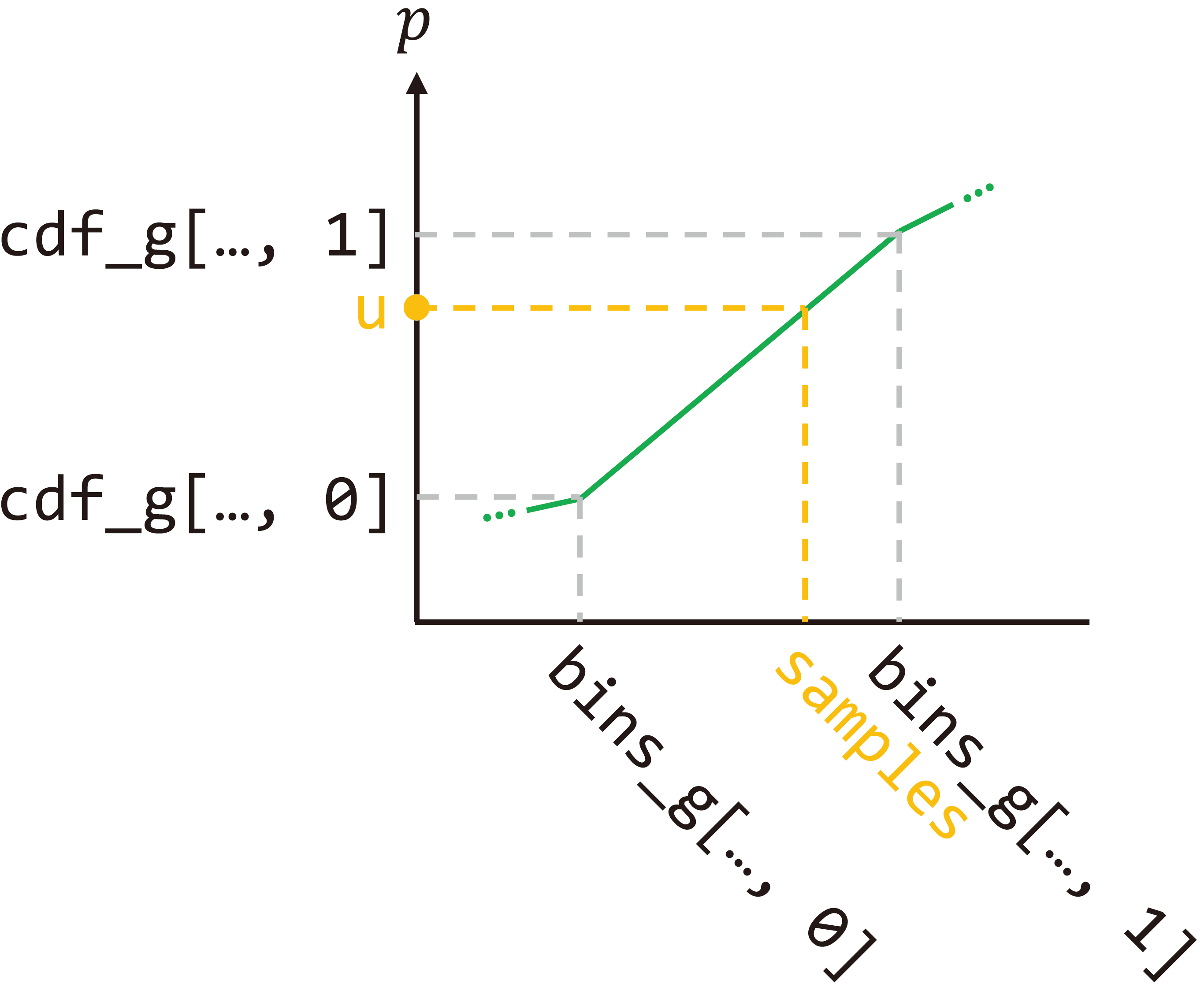
Finally, fine samples are found through similarity, whose concept is illustrated above. Indices 0 correspond to below, and indices 1 attach to above. Given cumulative probabilities u, there holds

$$\frac{\mathbf{u} - \verb|cdf[..., 0]|}{\verb|cdf[..., 1]| - \verb|cdf[..., 0]|} = \frac{\gray{\verb|z_|}\verb|samples| - \verb|bins_g[..., 0]|}{\verb|bins_g[..., 1]| - \verb|bins_g[..., 0]|}$$

Line $\verb|36|$ defines $\verb|denom| := \verb|cdf[..., 1]| - \verb|cdf[..., 0]|$, and line $\verb|39|$ further denotes $\mathbf{t}_{\gray{B \times N_F}} := \frac{\mathbf{u} - \verb|cdf[..., 0]|}{\verb|denom|}$, then

$$\mathbf{t}_{\gray{B \times N_F}} = \frac{\gray{\verb|z_|}\verb|samples| - \verb|bins_g[..., 0]|}{\verb|bins_g[..., 1]| - \verb|bins_g[..., 0]|}$$

Hence, lines $\verb|40|$ and $\verb|41|$ determine the unsorted output. Fine samples are expressed in offset from (midpoints of) coarse samples bins_g[..., 0].

$$\gray{\verb|z_|}\verb|samples| = \verb|bins_g[..., 0]| + \mathbf{t} * \left( \verb|bins_g[..., 1]| - \verb|bins_g[..., 0]| \right)$$

Optimization

    …
    for i in trange(start, N_iters):
        …
        optimizer.zero_grad()
        img_loss = img2mse(rgb, target_s)
        trans = extras['raw'][...,-1]
        loss = img_loss
        psnr = mse2psnr(img_loss)

        if 'rgb0' in extras:
            img_loss0 = img2mse(extras['rgb0'], target_s)
            loss = loss + img_loss0
            psnr0 = mse2psnr(img_loss0)

        loss.backward()
        optimizer.step()

        # NOTE: IMPORTANT!
        ###   update learning rate   ###
        decay_rate = 0.1
        decay_steps = args.lrate_decay * 1000
        new_lrate = args.lrate * (decay_rate ** (global_step / decay_steps))
        for param_group in optimizer.param_groups:
            param_group['lr'] = new_lrate
        ################################
        …

Radiance rgb $\in \mathbb{R}^{B \times 3}$ is compared against the ground truth target_s to obtain the MSE loss at line $\verb|5|$. The total loss also includes that of the coarse network (line $\verb|12|$). The coarse and fine network are jointly optimized at lines $\verb|15|$ and $\verb|16|$. Eventually, learning rate decays from line $\verb|20|$ to $\verb|24|$.

Summary

This post derives the volmue rendering integral and its numrical quadrature. Also explained is its connection with classical alpha compositing. The second part elaborates on the implementation of the rendering pipeline. Illustrations are included to assist understanding procedures such as rays generation and Monte Carlo sampling. Most importantly, the article clearly specifies the physical meaning of each variable and provides the mathematical operation for each statement. To sum, the blog functions as a complete guide for in-depth comprehension of NeRF.

References

Chapter 2.1 in Computer Vision: Algorithms and Applications
Foundamentals of Computer Graphics
NeRF: Representing Scenes as Neural Radiance Fields for View Synthesis
NeRF PyTorch implementation by Yen-Chen Lin
Neural Radiance Field's Volume Rendering 公式分析
Optical Models for Direct Volume Rendering
Part 1 of the SIGGRAPH 2021 course on Advances in Neural Rendering
深度解读yenchenlin/nerf-pytorch项目

Please use the following BibTeX to cite this post:

@misc{yyu2022nerfrendering,
    author = {Yu, Yue},
    title  = {NeRF: A Volume Rendering Perspective},
    year   = {2022},
    howpublished = {\url{https://yconquesty.github.io/blog/ml/nerf/nerf_rendering.html}}
}

Appendix

Content on the way. Stay tuned!

Errata

Time	Modification
Aug 31 2022	Initial release
Nov 24 2022	Rectify reference list
Dec 2 2022	Add BibTeX for citation
Apr 20 2023	Elaborate on static compute graph